Uncategorized
What Is OpenClaw (Formerly Clawdbot)? The Self-Hosted AI Assistant Explained
If you’ve been hearing about “Claw Bot AI” or “Clawdbot” and wondering what all the buzz is about, you’re not alone. OpenClaw — originally launched as Clawdbot, briefly renamed to Moltbot, and now officially called OpenClaw — has quickly become one of the most talked-about open-source AI projects of 2026. It represents a fundamentally different approach to AI assistants: one that runs on your own hardware, connects to your existing messaging apps, and actually takes action on your behalf.
In this guide, we’ll break down exactly what OpenClaw is, how it works, and why developers and power users are paying attention to it.
The Name Change History: Clawdbot to Moltbot to OpenClaw
Before we dive in, let’s clear up the naming confusion. The project was originally published in November 2025 by Austrian developer Peter Steinberger under the name Clawdbot (a play on Anthropic’s AI model “Claude”). In January 2026, Anthropic issued a trademark complaint because the name sounded too similar to “Claude,” so the project was renamed to Moltbot — keeping the lobster mascot theme. Just days later, it was renamed again to OpenClaw, which is the current and official name.
If you see references to Clawdbot, Moltbot, Claw Bot AI, or OpenClaw online, they’re all referring to the same project. The CLI command has transitioned to openclaw, though some older tutorials still reference the previous names.
What OpenClaw Actually Does
Most AI assistants you’ve used — ChatGPT, Siri, Google Assistant — are fundamentally reactive. You ask a question, they give an answer. They live in the cloud, they forget you when you close the tab, and they can’t actually do anything on your computer.
OpenClaw is different in several key ways:
It runs locally on your machine. OpenClaw installs on your own computer or server. Your data, conversation history, and configuration files stay on your hardware. Nothing is sent to external servers unless you explicitly tell it to (like sending an email or calling a cloud AI model).
It connects to your existing messaging apps. Instead of a separate app or browser tab, you interact with OpenClaw through the messaging platforms you already use — WhatsApp, Telegram, Discord, Slack, Signal, iMessage, and more. You message it like you’d message a coworker.
It actually takes action. OpenClaw can clear your inbox, send emails, manage your calendar, check you in for flights, organize files, run shell commands, automate browser tasks, and control smart home devices. It’s not just answering questions — it’s doing work.
It runs 24/7 in the background. Once set up as a background service (daemon), OpenClaw stays active even when you close your terminal. It can run scheduled tasks (cron jobs), send you proactive reminders, and monitor systems while you’re away.
It remembers everything. OpenClaw maintains persistent memory across sessions. Your preferences, past conversations, and context carry over, so you never have to repeat yourself.
How OpenClaw Works Under the Hood
OpenClaw itself is not a large language model. It’s an orchestration layer — a gateway that connects an AI model of your choice to your local system and messaging platforms. Think of it as the “brain and hands” architecture:
The “Brain” is whichever AI model you connect — Claude (from Anthropic), GPT-4 (from OpenAI), Gemini (from Google), or even local models running through Ollama for fully private inference. The brain handles reasoning and natural language understanding.
The “Hands” are OpenClaw’s execution environment — the skills, shell access, file management, browser automation, and messaging integrations that let the AI actually interact with your computer and the outside world.
Your workspace directory (typically ~/.openclaw/) stores configuration, memory files, credentials, and the agent’s personality profile (defined in a file called SOUL.md).
What Can You Do With OpenClaw?
The range of practical use cases is surprisingly broad. People are using OpenClaw for email management (inbox triage, drafting responses), calendar scheduling, file organization, browser automation like booking flights and filling out forms, running shell commands, smart home control, expense tracking, and even autonomous coding workflows when paired with tools like Claude Code.
OpenClaw also supports custom “skills” — modular plugins you can install from ClawHub (the community skill registry) or build yourself. Skills extend what the agent can do, from web search to API integrations to specialized automation tasks.
For a deeper look at practical examples, check out our guide to 10 things you can do with OpenClaw.
Supported Platforms
OpenClaw runs on macOS, Windows (via WSL2), and Linux. macOS is often considered the best platform for OpenClaw because the project was largely built for the Apple ecosystem, with native features like a menu bar companion app, Voice Wake (“Hey Claw”), and iMessage integration.
Windows users need to run OpenClaw through WSL2 (Windows Subsystem for Linux), as native Windows is not officially supported. Linux works natively and is ideal for headless servers, VPS deployments, or Raspberry Pi setups.
If you’re ready to get started, we have dedicated installation guides:
How to install OpenClaw on Windows (WSL2 guide)
How to install OpenClaw on Mac
How to install OpenClaw on DigitalOcean
Is OpenClaw Free?
Yes. OpenClaw is completely free and open-source under the MIT license. The software itself costs nothing. The only expense is the API usage cost for whichever AI model you connect — for example, if you use Claude or GPT-4, you’ll pay based on your provider’s token pricing. If you run a local model through Ollama, the entire setup is completely free (aside from electricity and hardware).
The Security Question
Because OpenClaw has access to your file system, shell, messaging accounts, and potentially your email and calendar, security is a real consideration. The project includes several built-in safeguards: a pairing system that requires approval before unknown users can message your bot, loopback binding so the gateway isn’t exposed to your network by default, gateway authentication tokens, sandboxed execution for non-main sessions, and configurable consent prompts before write or execute commands.
That said, cybersecurity researchers have raised concerns. Running an AI agent with broad system access creates a real attack surface, particularly around untrusted community skills and prompt injection risks. We cover this topic thoroughly in our OpenClaw security guide.
Who Is OpenClaw For?
OpenClaw is best suited for developers, power users, and technically-minded people who are comfortable with the command line. The setup requires working with terminal commands, API keys, and configuration files. As one of the project’s own maintainers put it, if you can’t understand how to run a command line, this may be too advanced of a tool to use safely.
If you’re a developer looking for an always-on AI assistant that respects your privacy and can actually execute tasks, OpenClaw is worth exploring. If you’re looking for a plug-and-play consumer product, it’s not quite there yet.
The Future of OpenClaw
In February 2026, Peter Steinberger announced he would be joining OpenAI, and the OpenClaw project will be moved to an open-source foundation. The community of over 84,000 developers continues to grow, and the project has collected significant traction on GitHub. Whether OpenClaw itself becomes the dominant personal AI agent or simply proves the concept that others build on, it represents a meaningful shift in how we think about AI — from tools that answer questions to agents that take action.
Related Guides on Code Boost
How to Install OpenClaw on Windows (Step-by-Step WSL2 Guide)
How to Install OpenClaw on Mac (macOS Setup Guide)
How to Install OpenClaw on DigitalOcean (Cloud VPS Guide)
Should You Run OpenClaw on Your Own Machine — or One You Don’t Own?
When people ask whether they should install OpenClaw locally or on a remote server, they’re usually thinking about cost or convenience.
But that’s not the real question.
The real question is:
If something goes wrong, how much of your life does it touch?
That’s what this decision is actually about — control, isolation, and blast radius.
Let’s break it down clearly.
First: What Does OpenClaw Actually Do?
Before we compare environments, we need to understand capability.
Depending on your setup, OpenClaw may:
-
Execute shell commands
-
Write and modify files
-
Store API keys (OpenAI, Stripe, Meta, etc.)
-
Receive webhooks from external services
-
Run continuously in the background
-
Integrate with Git repos
-
Process user input
That means it isn’t just a dashboard.
It’s an automation surface.
And anything that can execute logic, store secrets, or interact with external systems deserves thoughtful placement.
Option 1: Running OpenClaw on Your Own Machine
This usually means:
-
Your laptop
-
Your desktop
-
A home server
-
A NAS
-
A local Docker setup
✅ Advantages
1. Full Physical Control
You own the hardware.
You control the disk.
You control the network.
No third-party provider involved.
2. No Hosting Cost
No monthly bill.
No droplet to manage.
3. Fast Local Development
Lower latency.
Easy debugging.
Quick iteration.
4. Not Publicly Exposed (If LAN-Only)
If you don’t port-forward, it stays internal.
That’s a very strong security baseline.
❌ Risks
Here’s where it gets real.
If OpenClaw runs on your primary machine, it may have access to:
-
~/.sshkeys -
Browser cookies
-
Saved sessions
-
Local databases
-
Git repos
-
Mounted NAS drives
-
Terminal history
-
Environment files with API keys
-
Your entire home directory
Even if you didn’t intend that.
Operating systems don’t naturally sandbox apps the way people assume.
If OpenClaw (or something interacting with it):
-
Executes unexpected code
-
Pulls a malicious plugin
-
Has a vulnerability exploited
-
Accepts unsafe user input
Then the compromise isn’t isolated to a “tool.”
It’s your actual machine.
The Key Concept: Blast Radius
Blast radius =
How much damage can occur if this thing is compromised?
Compare:
| Deployment | Blast Radius |
|---|---|
| Local workstation | Potentially your entire user environment |
| Dedicated home server | Everything on that server |
| Isolated VM in cloud | Only that VM |
| Container with limited mounts | Even smaller |
This is the architectural lens most people miss.
The question isn’t:
“Is cloud safer?”
It’s:
“How much can this tool touch?”
Option 2: Running OpenClaw on a Machine You Don’t Own (Cloud)
This could mean:
-
A DigitalOcean droplet
-
An AWS EC2 instance
-
A VPS
-
Any minimal remote Linux server
Let’s reframe something important:
You are not giving up control.
You are containing access.
✅ Advantages
1. Clean Environment
A fresh cloud VM has:
-
No smart TV
-
No NAS
-
No browser sessions
-
No personal SSH keys
-
No unrelated services
It’s minimal.
That’s powerful.
2. Reduced Blast Radius
If compromised:
-
You destroy the VM
-
Rotate keys
-
Rebuild
Your laptop?
Untouched.
Your Synology?
Untouched.
Your personal GitHub access?
Untouched.
Isolation is everything.
3. Stronger Network Controls
Cloud providers allow:
-
Firewall rules at provider level
-
Restricting SSH to your IP
-
Only exposing ports 80/443
-
Easy TLS via reverse proxy
Most home routers do not provide this level of control.
4. Designed to Be Internet-Facing
If OpenClaw:
-
Receives webhooks
-
Handles OAuth callbacks
-
Needs uptime
-
Is accessed remotely
Cloud infrastructure is built for that.
Home networks are not.
❌ Tradeoffs
This isn’t a magic solution.
-
It costs money
-
It requires configuration
-
It is publicly reachable
-
It will be scanned constantly
Cloud security failures are usually misconfiguration issues.
But those risks are typically more manageable than unrestricted local access.
The Real Security Question
Ask yourself:
What does OpenClaw need access to?
If it needs:
-
Production API keys
-
Payment integrations
-
Advertising tokens
-
Git credentials
-
Long-running background execution
-
External webhooks
Then isolation becomes extremely important.
If it’s:
-
Personal experimentation
-
Offline workflows
-
Development only
-
No stored secrets
Local may be perfectly reasonable.
A Common Mistake: Local + Port Forwarding
This is the worst of both worlds.
-
Public exposure
-
Consumer router
-
No provider-level firewall
-
Often no TLS
-
No monitoring
If you’re going to expose it publicly, do it properly — and cloud environments make that easier.
The Professional Model
In production environments, tools like OpenClaw are typically:
-
Containerized
-
Run as non-root user
-
Given minimal file system mounts
-
Provided scoped API keys
-
Firewalled tightly
-
Monitored
-
Backed up
This is easier to achieve cleanly in a dedicated remote VM than on your daily-use machine.
When You Should Run It Locally
-
Development and testing
-
No public exposure
-
No sensitive stored secrets
-
You fully understand Docker isolation
-
You control network segmentation
When You Should Run It on a Remote Server
-
Handling production API keys
-
Receiving webhooks
-
Interacting with money (Stripe, ads, etc.)
-
Multi-user access
-
Long-running automations
-
Anything business-critical
The Hybrid Model (Often the Best Choice)
Many experienced builders do this:
-
Develop locally
-
Deploy to cloud for production
-
Keep environments separate
-
Use different API keys per environment
-
Limit permissions aggressively
This gives speed and isolation.
Final Thought: It’s About Containment, Not Ownership
Running OpenClaw on a machine you don’t own isn’t about trust.
It’s about control.
When you run it locally, you are granting it implicit access to your world.
When you run it in a clean, isolated environment, you are choosing exactly what it can touch — and nothing more.
That difference is the entire conversation.
And once you think in terms of blast radius instead of convenience, the deployment decision becomes much clearer.
Heroku in Maintenance Mode – Why We’re Not Building New Projects on Heroku (And What We’re Choosing Instead)
Heroku is not shutting down.
It remains supported, secure, and operational. Existing applications continue to run without disruption.
However, Salesforce has shifted Heroku into a sustaining engineering model. That shift changes how we evaluate it for new infrastructure decisions.
This article explains:
-
What Heroku’s maintenance mode really means
-
Whether it’s safe to build new projects on Heroku
-
The long-term risks developers should consider
-
Modern Heroku alternatives in 2026
-
A practical decision framework
If you’re deciding whether to build on Heroku in 2026, this guide will help.
What Changed With Heroku?
Salesforce repositioned Heroku into a maintenance-focused strategy:
-
Security updates continue
-
Stability is maintained
-
Compliance support remains
-
Critical bug fixes continue
-
Major feature innovation has slowed
-
Enterprise growth investment has cooled
This is not a shutdown.
But it is a trajectory change.
What “Maintenance Mode” Means for Developers
A platform in sustaining engineering typically focuses on:
| Area | Expected Status |
|---|---|
| Security patches | Continue |
| Stack updates (Ubuntu LTS) | Continue |
| Runtime support (Node, Ruby, etc.) | Continue, but conservatively |
| Major new features | Limited |
| New compute types (GPU/ARM) | Unlikely |
| Ecosystem expansion | Slower |
| Marketplace innovation | Gradual decline risk |
Heroku is now optimized for stability, not expansion.
That distinction matters for long-term architecture planning.
Is Heroku Safe to Use in 2026?
Yes — for existing applications.
The more important question is:
Should you build new projects on Heroku?
That depends on your goals.
Heroku: Strengths and Limitations
Strengths
-
Extremely simple deployment workflow
-
Mature operational stability
-
Strong historical documentation
-
Good fit for small SaaS and internal tools
-
Minimal DevOps overhead
Limitations
-
Slower platform innovation
-
Limited roadmap visibility
-
Potential ecosystem contraction over time
-
Less differentiation in a container-native world
-
Higher lock-in via add-ons and workflows
Heroku vs Modern Alternatives (Comparison)
Here’s a high-level comparison for new builds:
| Feature / Criteria | Heroku | Render | Fly.io | Railway | DigitalOcean App Platform | DigitalOcean (Droplets + Docker) |
|---|---|---|---|---|---|---|
| Platform Status | Maintenance mode | Actively expanding | Actively expanding | Actively expanding | Actively expanding | Fully developer-controlled |
| Deployment Model | Git-based + buildpacks | Git + Docker | Docker-first | Git + Docker | Git + Docker | Docker / manual |
| Container Native | Partial | Yes | Yes | Yes | Yes | Yes |
| Roadmap Velocity | Low | Medium–High | High | Medium | Medium–High | Depends on you |
| GPU Support | No | Limited | Emerging edge focus | No | Limited | Yes (via DO GPU droplets) |
| Edge / Multi-Region | Limited | Moderate | Strong global edge | Limited | Moderate | Manual setup |
| Managed Databases | Yes | Yes | Yes | Yes | Yes | Yes (separate product) |
| Add-On Marketplace | Mature but static | Growing | Smaller | Growing | Smaller | External services |
| Vendor Lock-In Risk | Moderate–High | Moderate | Moderate | Moderate | Moderate | Low |
| Infra Control | Low | Moderate | Moderate | Moderate | Moderate | High |
| DevOps Required | Very Low | Low | Moderate | Low | Low | Moderate–High |
| Long-Term Scalability | Stable plateau | Growing | Growing | Growing | Growing | Fully scalable (manual) |
| Best For | Legacy apps, simple SaaS | Modern SaaS | Edge apps, global scale | Fast MVP | Simpler PaaS w/ cloud flexibility | Full control, cost efficiency |
Key Insight:
Heroku remains stable. Most alternatives are still investing and expanding.
The Lock-In Factor
One of the most overlooked considerations is migration difficulty.
Heroku encourages platform-native workflows:
-
Buildpacks
-
Release phase
-
Add-ons marketplace
-
Platform-managed config vars
-
Review apps and pipelines
These accelerate early development.
They can increase migration friction later.
Lock-In Spectrum
| Lock-In Level | Example Setup | Migration Difficulty |
|---|---|---|
| Low | Dockerized app + external DB | Low |
| Medium | Heroku Postgres + buildpacks | Moderate |
| High | Heavy add-ons + pipelines + release workflows | High |
Before committing to Heroku for a new system, ask:
If we needed to migrate in 24 months, how painful would this be?
The Bigger Industry Context
When Heroku became dominant:
-
Containers were not universal
-
CI/CD tooling was immature
-
Infrastructure automation was niche
-
Platform engineering was rare
In 2026:
-
Docker is standard
-
Managed container platforms are abundant
-
Infrastructure as Code is expected
-
Portability is a priority
Heroku’s original abstraction advantage has narrowed.
It is no longer uniquely differentiated.
Our Decision Framework
We use a simple infrastructure evaluation checklist.
We Avoid Platforms That:
-
Are in maintenance mode
-
Have limited roadmap transparency
-
Show declining ecosystem momentum
-
Introduce hard-to-reverse architectural lock-in
We Prefer Platforms That:
-
Are container-native
-
Actively expanding features
-
Support portability
-
Align with cloud-native standards
Decision Matrix: Should You Use Heroku in 2026?
| Scenario | Recommendation |
|---|---|
| Existing stable app | Stay |
| Small MVP / side project | Acceptable |
| Funded startup planning 3–5 years | Consider alternatives |
| Compliance-heavy enterprise system | Consider alternatives |
| Long-term scalable SaaS | Use growth-aligned platform |
| Need GPU / edge / infra flexibility | Choose alternative |
What We’re Choosing Instead
We are prioritizing platforms that are:
-
Container-first
-
Actively developed
-
Portable
-
Transparent about roadmap direction
Depending on project complexity, that includes:
-
Modern managed PaaS platforms
-
Cloud-native container services
-
Kubernetes for advanced workloads
-
Docker + VPS for controlled deployments
The consistent theme is momentum + portability. For this we like DigitalOcean.
Frequently Asked Questions About Heroku in 2026
Is Heroku shutting down?
No. It remains operational and supported.
Is Heroku still secure?
Yes. Security patches and compliance updates continue.
Should I migrate immediately?
Not necessarily. Existing apps can remain stable.
Is it wise to start a new SaaS on Heroku?
It depends. For short-term simplicity, possibly. For long-term infrastructure strategy, alternatives may offer more growth alignment.
What are the best Heroku alternatives?
Popular options include modern managed PaaS platforms and cloud-native container services that continue active development.
Final Thoughts
Heroku in 2026 is:
-
Stable
-
Supported
-
Mature
It is not:
-
Rapidly expanding
-
Aggressively innovating
-
Positioned as a strategic growth engine
For existing systems, stability may be enough.
For new builds, we prefer platforms aligned with forward momentum.
Infrastructure decisions compound.
We choose to build where innovation is still accelerating.
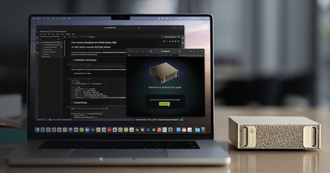
How to Combine a DGX Spark and Mac Studio Into One Fast AI Inference Machine (And Why It Works)
There’s a setup quietly circulating in AI developer circles that sounds almost too good to be true: take an NVIDIA DGX Spark ($3,999), wire it to an Apple Mac Studio ($5,599), and get nearly 3× the inference speed you’d get from either machine alone.
It’s real. EXO Labs demonstrated it. The benchmarks hold up. And the underlying principle — called disaggregated inference — is the same architecture NVIDIA is building into its next-generation data center hardware.
This post explains exactly why this works, what you need, how compatible it is with hardware you might already own, and how to think about whether it’s worth pursuing for your own local AI setup.
The Core Idea: Each Machine Is Good at a Different Thing
Every time you send a prompt to a large language model, two very different phases happen under the hood.
Phase 1 — Prefill. The model reads your entire prompt and builds an internal state called the KV cache. This phase is compute-heavy. It involves massive matrix multiplications across every transformer layer. The longer your prompt, the more compute it demands — it scales quadratically with token count. What matters here is raw GPU compute power (FLOPS).
Phase 2 — Decode. The model generates tokens one at a time. Each new token needs to read the entire KV cache to figure out what comes next. This phase is memory-bandwidth-heavy. There’s less math, but the model needs to shuttle large amounts of data from memory to the GPU constantly. What matters here is memory bandwidth (GB/s).
Here’s the thing: the DGX Spark and the Mac Studio are almost perfectly mismatched in these two dimensions.
| DGX Spark | Mac Studio M3 Ultra | |
|---|---|---|
| FP16 Compute | ~100 TFLOPS | ~26 TFLOPS |
| Memory Bandwidth | 273 GB/s | 819 GB/s |
| Unified Memory | 128 GB | Up to 512 GB |
| Price | $3,999 | ~$5,599 (256GB config) |
The Spark has 4× the compute but only one-third the memory bandwidth of the Mac Studio. The Mac Studio has 3× the bandwidth but only one-quarter the compute.
So what if you ran prefill on the Spark (where compute matters) and decode on the Mac Studio (where bandwidth matters)?
That’s exactly what disaggregated inference does. And it’s exactly what EXO automates.

The Benchmark That Proves It
EXO Labs ran Llama 3.1 8B (FP16) with an 8,192-token prompt, generating 32 output tokens. Here are the results:
| Setup | Prefill Time | Decode Time | Total Time | Speedup |
|---|---|---|---|---|
| DGX Spark alone | 1.47s | 2.87s | 4.34s | 1.9× |
| Mac Studio M3 Ultra alone | 5.57s | 0.85s | 6.42s | 1.0× (baseline) |
| Spark + Mac Studio (EXO) | 1.47s | 0.85s | 2.32s | 2.8× |
The hybrid setup takes the best number from each column. The Spark’s prefill speed (3.8× faster than the Mac) combined with the Mac’s decode speed (3.4× faster than the Spark) delivers a combined result that’s 2.8× faster than the Mac alone and 1.9× faster than the Spark alone.
Neither machine can achieve this on its own. The combination is genuinely greater than the sum of its parts.
Click Here To Learn More About DGX Spark
How the KV Cache Transfer Actually Works
The obvious question: doesn’t sending the KV cache from one machine to the other add a huge delay?
It would, if you did it the naive way — finish all prefill, transfer the entire KV cache as one blob, then start decode. For a large model, that transfer could take seconds.
EXO solves this by streaming the KV cache layer by layer, overlapping the transfer with ongoing computation. Here’s the sequence:
- The Spark completes prefill for Layer 1
- Simultaneously: Layer 1’s KV cache starts streaming to the Mac Studio AND the Spark begins prefill for Layer 2
- By the time all layers are done, most of the KV cache has already arrived at the Mac Studio
- Decode begins immediately on the Mac Studio
The math works out because prefill computation per layer (which scales quadratically with prompt length) takes longer than KV transfer per layer (which scales linearly). For models with grouped-query attention (GQA) like Llama 3 8B and 70B, full overlap is achievable with prompts as short as 5,000–10,000 tokens over a 10GbE connection. With older multi-head attention models, you need longer prompts (~40k+ tokens) for the overlap to fully hide the network latency.
In practical terms: if you’re processing documents, codebases, or long conversation histories — the exact workloads where you’d want large models — the overlap works in your favor.
What You Need to Build This
The Hardware
Minimum viable setup:
- 1× NVIDIA DGX Spark (any variant — Founders Edition, ASUS Ascent GX10, Dell Pro Max GB10, MSI EdgeXpert)
- 1× Apple Mac Studio with M3 Ultra (or any Apple Silicon Mac with substantial unified memory)
- 1× 10GbE Ethernet connection between the two machines
About the network connection: Both the DGX Spark and the Mac Studio M3 Ultra have 10GbE Ethernet ports built in. You just need a Cat6a or Cat7 Ethernet cable between them — either direct (point-to-point) or through a 10GbE switch. No special networking hardware beyond what’s already in the boxes. The Spark also has its ConnectX-7 200GbE QSFP ports, but the EXO setup uses standard 10GbE, which both machines support natively.
Expanded setup (what EXO Labs tested):
- 2× DGX Sparks (connected together via ConnectX-7 for additional compute)
- 1× Mac Studio M3 Ultra (256GB unified memory)
- 10GbE network between all devices
The Software: EXO
EXO is an open-source framework from EXO Labs that turns any collection of devices into a cooperative AI inference cluster. It handles device discovery, model partitioning, KV cache streaming, and phase placement automatically.
Key facts about EXO:
- Open source: github.com/exo-explore/exo
- Supports NVIDIA GPUs (CUDA), Apple Silicon (MLX), and even CPUs
- Automatic device discovery — devices on the same network find each other without manual configuration
- ChatGPT-compatible API — your existing code that calls OpenAI-style endpoints works with a one-line URL change
- Built-in web dashboard for model management and chat
- Peer-to-peer architecture — no master/worker hierarchy
Current status (important caveat): The disaggregated inference features shown in the DGX Spark + Mac Studio demo are part of EXO 1.0. As of late 2025, EXO’s public open-source release (0.0.15-alpha) supports basic model sharding and multi-device inference, but the full automated prefill/decode splitting with layer-by-layer KV streaming is a newer capability. Check the GitHub repo for the latest release status.
Installation
On the Mac Studio (macOS):
# EXO can be installed via Homebrew or from source
brew install exo

# Or from source:
git clone https://github.com/exo-explore/exo.git
cd exo
pip install -e .

# Optimize Apple Silicon GPU memory allocation
./configure_mlx.sh
On the DGX Spark (DGX OS / Ubuntu):
git clone https://github.com/exo-explore/exo.git
cd exo
pip install -e .
Then, on both machines:
exo
That’s it. EXO discovers the other device automatically, profiles each device’s compute and bandwidth capabilities, and determines the optimal way to split the workload. A web dashboard launches at http://localhost:52415 where you can download models and start chatting.
Compatibility: What Hardware Can You Actually Use?
This is the question most people have. Let’s break it down.
Do you already own a Mac Studio, MacBook Pro, or Mac Mini?
Yes, you can use it. EXO supports any Apple Silicon device — M1 through M4 Ultra. The benefit scales with your memory configuration:
- Mac Mini M4 Pro (24GB): Useful for small models. Limited as a decode node for large models.
- MacBook Pro M4 Max (64–128GB): Solid decode node. Good bandwidth (~546 GB/s on M4 Max).
- Mac Studio M3/M4 Ultra (192–512GB): Ideal decode node. Highest bandwidth in the Apple lineup (~819 GB/s on M3 Ultra).
The key metric is memory bandwidth. The more bandwidth your Mac has, the faster it handles the decode phase.
Do you need specifically a DGX Spark for the compute node?
No, but it’s the best fit. The DGX Spark’s advantage is its Blackwell Tensor Cores with FP4 support, which deliver exceptional prefill throughput for its power envelope. But EXO supports any NVIDIA GPU with CUDA. In principle:
- A desktop with an RTX 4090 or 5090 could serve as the prefill node
- A Linux machine with any CUDA-capable GPU can participate
- The benefit is proportional to the GPU’s compute throughput
The Spark’s specific advantage is that it has high compute AND 128GB of unified memory, meaning it can prefill large models without running out of VRAM — something a 24GB RTX 4090 can’t do for 70B models.
What about networking?
- 10GbE (recommended minimum): Both the DGX Spark and Mac Studio have built-in 10GbE. This provides enough bandwidth for layer-by-layer KV streaming on most models with prompts over ~5k tokens.
- Thunderbolt 5 with RDMA: EXO now supports RDMA over Thunderbolt 5 on compatible Macs (M4 Pro Mac Mini, M4 Max Mac Studio, M4 Max MacBook Pro, M3 Ultra Mac Studio). This reduces inter-device latency by 99% compared to TCP/IP networking. Requires matching macOS versions on all devices.
- Standard 1GbE: Works for basic model sharding but will bottleneck KV streaming for the disaggregated inference setup. Not recommended for the Spark + Mac hybrid workflow.
- Wi-Fi: EXO supports it for device discovery and basic inference, but the bandwidth is too low for competitive disaggregated inference speeds.
Can you use this with models other than Llama?
Yes. EXO supports LLaMA, Mistral, Qwen, DeepSeek, LLaVA, and others. The disaggregated inference benefit applies to any transformer-based model, though the specific crossover point (where KV transfer overlaps fully with compute) depends on the model’s attention architecture. Models with grouped-query attention (GQA) — which includes most modern large models — benefit at shorter prompt lengths.
Who This Setup Is Actually For
Developers and researchers who already own both an NVIDIA GPU system and an Apple Silicon Mac. If you already have a Mac Studio for daily work and you’re considering a DGX Spark for CUDA development, the hybrid cluster is a compelling bonus. Instead of choosing between them, you use both together.
Teams running RAG pipelines with long context. The disaggregated approach shines with long input prompts (5k+ tokens). If your workflow involves ingesting documents, codebases, or knowledge bases before generating responses, the Spark handles that ingestion phase at maximum speed while the Mac generates the actual output at maximum bandwidth.
Anyone frustrated by the “compute vs. bandwidth” trade-off. Every current AI device forces a compromise. High-end NVIDIA GPUs have incredible compute but limited VRAM. Apple Silicon has massive bandwidth but modest compute. The hybrid cluster sidesteps this trade-off entirely by using each device for the phase it’s optimized for.
Who this is probably NOT for
Casual users running 7B models. If your models fit comfortably on a single device and generate tokens fast enough for your needs, the complexity of a multi-device setup isn’t worth it.
Anyone expecting plug-and-play simplicity today. EXO is actively evolving. The basic multi-device inference works well. The advanced disaggregated scheduling is newer. Expect some configuration and troubleshooting, particularly around network optimization and model compatibility.
Budget-constrained buyers. A DGX Spark ($4,000) plus a Mac Studio M3 Ultra ($5,600) is a $9,600+ investment. If cost is the primary concern, you’d get more raw tokens-per-dollar from a multi-GPU desktop build (though you’d lose the disaggregated inference benefit and the Apple development experience).
Click Here To Learn More About DGX Spark
The Bigger Picture: Why This Matters
This isn’t just a clever hack. Disaggregated inference — separating prefill and decode onto different hardware — is the same architectural principle NVIDIA is building into its next-generation data center platforms. NVIDIA’s upcoming Rubin CPX architecture will use compute-dense processors for prefill and bandwidth-optimized chips for decode, exactly mirroring what EXO demonstrates with off-the-shelf hardware today.
The implications are significant:
Your hardware doesn’t have to be one brand. The DGX Spark runs CUDA on ARM Linux. The Mac Studio runs MLX on macOS. They speak to each other over standard Ethernet. The idea that your AI infrastructure has to be homogeneous is simply not true anymore.
Adding devices makes the system faster, not just bigger. Traditional multi-GPU setups often suffer from coordination overhead. Disaggregated inference is different — each device does what it’s best at, and the pipeline is additive rather than averaging.
This is early. EXO is experimental. The software is evolving rapidly. But the principle is sound, the benchmarks are real, and the trend in AI hardware is clearly moving toward heterogeneous, disaggregated architectures.
If you have a DGX Spark and a Mac Studio sitting on the same desk — or if you’re considering buying one to complement the other — it’s worth an afternoon of experimentation. The 2.8× speedup isn’t theoretical. It’s waiting for you on the other end of a 10GbE cable.
Quick Reference: What to Buy, What to Know
| Component | Recommendation | Why |
|---|---|---|
| Compute node | DGX Spark (any OEM variant) | Best prefill throughput per watt; 128GB handles large models |
| Bandwidth node | Mac Studio M3 Ultra 256GB+ | Highest memory bandwidth available in desktop form factor |
| Network | 10GbE Ethernet (built into both devices) | Sufficient for KV streaming; zero additional hardware cost |
| Software | EXO (github.com/exo-explore/exo) | Handles discovery, partitioning, and KV streaming automatically |
| Upgrade path | Thunderbolt 5 RDMA (if supported) | 99% latency reduction for Mac-to-Mac or Mac-to-Spark links |
| Models | GQA-based (Llama 3, Qwen 2.5, DeepSeek) | Better overlap efficiency at shorter prompt lengths |
| Sweet spot | Prompts 5k–128k tokens, 70B+ models | Where disaggregated inference provides the most dramatic gains |
Click Here To Learn More About DGX Spark
The NVIDIA DGX Spark: An Honest Technical Guide for AI Builders
Click Here For Latest Pricing
The NVIDIA DGX Spark is the first desktop hardware to put the full NVIDIA DGX software stack — previously exclusive to six-figure data center systems — into a 1.1-liter box that powers via USB-C. At $3,999 for the 4TB Founders Edition (or ~$3,000 from partners like ASUS with 1TB storage), it occupies a genuinely new category in AI hardware.
But “new category” doesn’t mean “right for everyone.” After months of community benchmarks, developer forum discussions, and independent reviews, a much clearer picture has emerged of what the DGX Spark actually does well, where it struggles, and who should seriously consider buying one.
This guide cuts through both the marketing hype and the reactionary criticism to give you a grounded, technical assessment.
What You’re Actually Getting: Hardware at a Glance
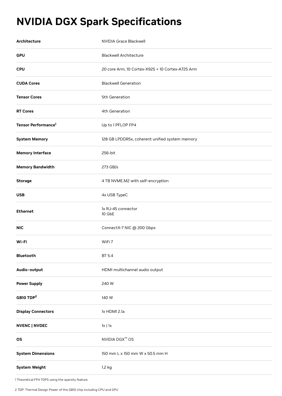
At the heart of the DGX Spark is the GB10 Grace Blackwell Superchip — an ARM-based CPU (10 Cortex-X925 + 10 Cortex-A725 cores) connected via NVLink-C2C to a Blackwell-generation GPU with 5th-gen Tensor Cores and native FP4 support.
The specs that matter:
- 128GB unified LPDDR5X memory — shared coherently between CPU and GPU, no PCIe transfer bottleneck
- 273 GB/s memory bandwidth — this is the number that defines real-world inference speed (more on this below)
- Up to 1 PFLOP of FP4 AI compute (with structured sparsity — the caveat matters)
- 6,144 CUDA cores — comparable to an RTX 5070-class GPU
- ConnectX-7 200GbE networking — two Sparks can cluster for models up to ~405B parameters
- ~240-300W total system power via USB-C
- DGX OS (Ubuntu-based) pre-installed with CUDA, cuDNN, TensorRT, NCCL, PyTorch, and NVIDIA’s full AI software stack
- NVMe storage: 1TB or 4TB options
Full Spec Sheet:
The unified memory architecture is the defining feature. Unlike a discrete GPU setup where 24GB of VRAM sits behind a PCIe bus separated from system RAM, the Spark’s entire 128GB memory pool is directly accessible by both the CPU and GPU. This eliminates the data transfer overhead that plagues consumer GPU workflows and is the reason a 70B model that won’t fit on an RTX 4090 loads directly into memory on the Spark.
Click Here To Learn More About DGX Spark
Real-World Performance: What the Benchmarks Actually Show
This is where nuance matters enormously. The DGX Spark has a split personality in benchmarks, and understanding why will tell you whether it fits your workflow.
Where It’s Genuinely Strong: Prompt Processing (Prefill)
The Blackwell GPU’s tensor cores shine during the compute-bound prefill phase — processing your input prompt before generating a response. Independent benchmarks from the llama.cpp community show impressive numbers:
- GPT-OSS 120B (MXFP4): ~1,725–1,821 tokens/sec prompt processing
- Llama 3.1 8B (NVFP4): ~10,257 tokens/sec prompt processing
- Qwen3 14B (NVFP4): ~5,929 tokens/sec prompt processing
For context, that GPT-OSS 120B prefill speed is faster than a 3×RTX 3090 rig (~1,642 tokens/sec) and roughly 5× faster than an AMD Strix Halo system (~340 tokens/sec). If your workload involves ingesting large contexts — RAG pipelines, long document analysis, code review — the Spark handles the input processing phase exceptionally well.
Where It’s Honest-to-God Slow: Token Generation (Decode)
Here’s the reality check. Token generation — the part where you’re waiting for the model to type its response word by word — is memory-bandwidth-bound. And 273 GB/s, while respectable for LPDDR5X, is a fraction of what discrete GPUs offer.
The numbers are clear:
- GPT-OSS 120B: ~35–55 tokens/sec (depending on quantization and backend)
- Llama 3.1 8B: ~36–39 tokens/sec
- Qwen3-Coder-30B (Q4, 16k context): ~20–25 tokens/sec
- Llama 3.1 70B (FP8): ~2.7 tokens/sec decode
For comparison, a single RTX 5090 generates tokens 3–5× faster on models that fit in its 32GB VRAM, and a 3×RTX 3090 rig hits ~124 tokens/sec on the GPT-OSS 120B model. An Apple Mac Studio M3 Ultra with comparable unified memory capacity also has higher memory bandwidth (~819 GB/s) and generates tokens faster for decode-heavy workloads.
The practical implication: For interactive chat-style use with large models (70B+), the Spark works but feels noticeably slower than what you’d get from a high-end discrete GPU (on models that fit in VRAM) or a maxed-out Mac Studio. For a 120B reasoning model that generates 10k+ tokens per response, waiting at ~35–55 tokens/sec is fine. At 2.7 tokens/sec on a dense 70B in FP8, it’s painful.
Fine-Tuning: The Genuine Sweet Spot
This is where the Spark arguably justifies its existence most clearly. NVIDIA’s published benchmarks show:
- Llama 3.2 3B full fine-tune: ~82,739 tokens/sec peak
- Llama 3.1 8B LoRA: ~53,658 tokens/sec peak
- Llama 3.3 70B QLoRA (FP4): ~5,079 tokens/sec peak
The critical detail: none of these fine-tuning workloads run on a 32GB consumer GPU. QLoRA on a 70B model requires the full model weights in memory plus optimizer states and gradient buffers. The Spark’s 128GB unified memory makes this possible without renting cloud A100s. If you’re iterating on fine-tuned models — adapting them to domain-specific data, private codebases, or specialized tasks — the ability to run these jobs locally, overnight, without cloud billing ticking, is a legitimate advantage.
Dual-Spark Clustering
Two DGX Sparks connected via the ConnectX-7 200GbE interface can run models up to ~405B parameters. NVIDIA demonstrated the Qwen3 235B model achieving ~11.73 tokens/sec generation on the dual setup. The EXO Labs team even combined two Sparks with an M3 Ultra Mac Studio in a hybrid cluster, using the Sparks for prefill and the Mac for decode, achieving a 2.8× speedup over the Mac alone. Interesting for experimentation, though the dual-Spark bundle runs ~$8,000.
Click Here To Learn More About DGX Spark
The Caveats You Need to Know
Being helpful means being honest about the rough edges.
The “1 PFLOP” Marketing Number
NVIDIA’s headline performance figure assumes FP4 precision with structured sparsity — a technique that doubles effective throughput by skipping zero-value operations. Real-world workloads don’t always align with this ideal condition. The actual compute experience is more comparable to an RTX 5070-class GPU. This isn’t dishonest per se (the hardware does achieve those numbers in the right conditions), but it doesn’t map cleanly to most workloads today.
Thermal Behavior
The Spark packs significant compute into a tiny chassis. Multiple users have reported the device running very hot during sustained workloads, with some experiencing throttling or reboots during extended fine-tuning runs. This appears to be an active area of firmware optimization by NVIDIA. If you plan to run multi-day fine-tuning jobs, monitor thermals and ensure adequate ambient airflow around the device.
ARM64 Compatibility
The underlying ARM64 architecture (not x86) means occasional friction with software that assumes an x86 environment. Major frameworks (PyTorch, Hugging Face, llama.cpp, Ollama, vLLM) all support it, and NVIDIA ships playbooks for common setups. But some precompiled binaries may be missing, and niche libraries might need manual builds. The DGX OS smooths most of this, but it’s not zero-friction if you have a complex existing toolchain.
The mmap Bug
A well-documented issue: leaving memory-mapped file I/O (mmap) enabled dramatically increases model loading times — up to 5× slower in some cases. The fix is simple (use --no-mmap in llama.cpp, or equivalent flags in other engines), and NVIDIA has been improving this through kernel updates (6.14 brought major improvements, 6.17 further so). But it’s the kind of thing that trips up new users who don’t know to look for it.
Storage Burns Fast
Large model files in multiple formats (GGUF, safetensors, FP4, FP8) consume storage quickly. Users report burning through 1TB within weeks of active experimentation. The 4TB Founders Edition is worth the extra $1,000 if you plan to keep multiple large models on hand. Alternatively, use network storage, but that adds latency to model loading.
Who Should Seriously Consider This
Strong Fit
AI researchers and data scientists who need to fine-tune large models locally. If you’re regularly running LoRA/QLoRA jobs on 8B–70B models and currently renting cloud GPUs for each experiment, the Spark pays for itself in cloud savings within weeks to months. The ability to kick off a fine-tuning run at your desk overnight, without a billing clock, is genuinely valuable.
Teams working with sensitive data that can’t leave premises. Healthcare, legal, financial, and defense applications where sending data to cloud inference endpoints is architecturally unacceptable. The Spark’s pre-configured DGX OS and local inference stack means code and data never leave your network.
Developers building and testing RAG pipelines and multi-model systems. The 128GB unified memory lets you run an LLM, an embedding model, a reranker, and supporting infrastructure simultaneously. The strong prefill performance means large context ingestion for RAG is fast.
Students, educators, and researchers who want the full NVIDIA AI stack in a portable package. The pre-installed, validated software environment (CUDA, cuDNN, TensorRT, Jupyter, AI Workbench) eliminates days of driver configuration. It’s a functional slice of a data center that you can carry in a backpack.
Physical AI and robotics developers. Edge deployment scenarios, simulations, and digital twin workloads that need GPU compute in a small, low-power form factor.
Weaker Fit
Developers who primarily need fast interactive inference on small-to-medium models. If your main workload is running 7B–13B models for chat or code completion, a Mac Mini M4 Pro ($1,400) or an RTX 5090 ($2,000) delivers comparable or faster token generation at a lower price. The Spark’s advantage only materializes when you need the memory for models that don’t fit on those systems.
Production inference serving at scale. The Spark is a development and prototyping platform. If you need to serve hundreds of concurrent users, you need proper server infrastructure. NVIDIA positions the Spark as the place you build and validate before deploying to DGX Cloud or data center systems.
Users who need maximum token generation speed above all else. If decode throughput is your primary metric, the 273 GB/s memory bandwidth is simply not competitive with high-end discrete GPUs (RTX 5090 at 1,792 GB/s) or even the M3 Ultra Mac Studio (~819 GB/s) for models that fit in those systems’ memory.
The Competitive Landscape: How It Stacks Up
Understanding the Spark’s position requires comparing it against the realistic alternatives.
vs. Apple Mac Studio M4 Ultra (when available) / M3 Ultra
Apple’s unified memory architecture offers higher bandwidth (~819 GB/s on M3 Ultra), which translates to faster token generation for decode-heavy workloads. A maxed-out Mac Studio can be configured with 192GB+ unified memory. For pure inference throughput on large models, Apple silicon currently wins on tokens-per-second at similar price points.
The Spark’s advantage: the full NVIDIA CUDA ecosystem, native FP4 hardware acceleration (NVFP4/MXFP4), TensorRT integration, and seamless model portability to DGX Cloud and data center infrastructure. If your production pipeline runs on NVIDIA GPUs, developing on the Spark means zero code changes when you scale up. If you live in the MLX/Apple ecosystem, the Mac Studio is probably a better fit.
vs. RTX 5090 Desktop
The 5090 is 3–5× faster for inference on models that fit in 32GB VRAM, at roughly half the price. If your models are 13B or smaller (quantized), the 5090 is the clear winner for speed and value.
The Spark’s advantage: 128GB vs 32GB memory means it can run 70B–120B models that the 5090 physically cannot. Different tool for a different job.
vs. Multi-GPU Rigs (2–3× RTX 3090/4090)
Multi-GPU setups offer higher aggregate memory bandwidth and faster decode speeds. A 3×RTX 3090 rig delivers ~124 tokens/sec on GPT-OSS 120B vs the Spark’s ~38 tokens/sec.
The Spark’s advantages: dramatically smaller physical footprint, 170–240W vs 900W+, no PCIe multi-GPU coordination overhead, pre-configured software stack, and the Blackwell FP4 hardware support. It’s a trade-off between raw speed and operational simplicity.
vs. Cloud GPU Instances
A single A100-80GB cloud instance runs $2–4/hour. If you’re doing 4+ hours of compute daily, the Spark pays for itself within 2–6 months depending on your workload. The Spark also eliminates instance availability issues, startup latency, and data transfer concerns. But cloud instances offer access to H100s and multi-GPU configs that far exceed the Spark’s raw performance.
Practical Tips If You Buy One
Based on community experience from the NVIDIA developer forums and independent users:
- Use llama.cpp for single-user inference. It consistently offers the best performance on the Spark with the least overhead. Ollama is convenient but slightly slower. vLLM and TensorRT have steeper setup curves with marginal gains for single-user workloads.
- Always use
--no-mmap. Model loading is dramatically faster. Also use--flash-attnand set-ngl 999to fully load models onto the GPU. - Prefer MoE (Mixture of Experts) models for interactive use. Users report that GPT-OSS 120B (a MoE model) runs surprisingly fast, while dense models of similar size are much slower. MoE models only activate a fraction of parameters per token, making them a much better fit for the Spark’s bandwidth profile.
- Get the 4TB version. Model files are large. You’ll burn through 1TB faster than you think if you’re experimenting with multiple model sizes and quantization formats.
- Clear buffer cache before loading large models. The unified memory architecture can hold buffer cache that isn’t released automatically. Run
sudo sh -c 'echo 3 > /proc/sys/vm/drop_caches'before loading large models to ensure maximum available memory. - Use NVIDIA Sync for remote access. The DGX Dashboard provides remote JupyterLab, terminal, and VSCode integration. You can run the Spark headless on your network and connect from your laptop — a better workflow than connecting peripherals directly.
- Monitor thermals during long runs. Ensure adequate ventilation around the device, especially for multi-hour fine-tuning jobs.
The Bottom Line
The DGX Spark is not the fastest local inference device per dollar. It’s not trying to be. It’s the smallest, most integrated entry point into the NVIDIA DGX ecosystem — a development platform that lets you build on the same software stack that powers enterprise AI infrastructure, in a package you can carry in one hand.
Its genuine strengths are: 128GB unified memory for running and fine-tuning models that can’t fit on consumer GPUs, strong prefill performance for context-heavy workloads, the full pre-configured NVIDIA AI software stack, and a seamless path from local development to cloud/data center deployment.
Its genuine weaknesses are: token generation speed limited by 273 GB/s memory bandwidth, thermal constraints in the compact chassis, and a price point that’s hard to justify if your models fit comfortably on a $2,000 discrete GPU.
For AI builders who have genuinely outgrown 24–32GB of VRAM, who need to fine-tune large models locally, who work with data that can’t touch a cloud, or who need to develop on the same CUDA stack they’ll deploy on — the DGX Spark fills a real gap that didn’t have a clean answer before. Go in with calibrated expectations, and it’s a capable tool. Go in expecting data center performance in a desktop box, and you’ll be disappointed.
The most useful framing comes from the community itself: think of the DGX Spark not as a consumer device, but as a personal development cluster — a functional slice of a data center that fits on your desk and lets you iterate without cloud dependencies. For the right user, that’s exactly what was missing.
Click Here To Learn More About DGX Spark
Beyond the 24GB Ceiling: Why Serious AI Builders Are Outgrowing Consumer GPUs
There’s a moment every AI engineer hits eventually. You’ve downloaded the latest open-weight 70B model. You’ve quantized it down to 4-bit. You’ve tweaked every llama.cpp flag you can find. And then you watch your RTX 4090 — a $1,600 card that was supposed to be the pinnacle of consumer GPU power — choke on a 32k context prompt while your system fans scream at full RPM.
Welcome to the 24GB ceiling.
It’s not a theoretical limitation. It’s the concrete wall that separates tinkering with AI from building production-grade systems on local hardware. And if you’re reading this, you’ve probably already hit it.
This post is for developers, technical founders, and AI builders who have outgrown consumer GPU setups but don’t want to hand their models, their data, or their margins to a cloud provider. We’ll break down exactly why 24GB of VRAM falls apart for serious workloads, what the hidden memory costs are that nobody warns you about, and why an emerging category of hardware — compact, high-memory AI workstations — is becoming the missing piece for local-first AI development.
Why Bigger Models Break Consumer GPUs
The math is straightforward, but the implications are brutal.
A 70B parameter model at full FP16 precision requires approximately 140GB of memory just to hold the weights. Even at aggressive 4-bit quantization (GPTQ or AWQ), you’re looking at roughly 35–40GB. That’s already 50% beyond what a single RTX 4090 can address.
The standard workaround is multi-GPU setups. Two 4090s give you 48GB of VRAM, which technically fits a heavily quantized 70B model. But “fits” is doing a lot of heavy lifting in that sentence. Loading model weights into VRAM is only the beginning of what inference actually requires.
There’s the KV cache, attention computation overhead, intermediate activation tensors, and any batch processing state. Once you account for all of that, a 48GB dual-GPU rig running a 4-bit 70B model has almost zero headroom. You can run it, but you can’t actually use it for anything demanding.
And multi-GPU introduces its own tax. Unless you’re using NVLink (which consumer cards don’t support natively), tensor parallelism across PCIe lanes adds latency to every forward pass. You’re splitting the model across devices that communicate through a bus that was designed for graphics rendering, not the all-to-all communication patterns that transformer inference demands. Real-world throughput on dual-4090 setups frequently disappoints engineers who expected near-linear scaling.
Then there’s the quantization trade-off itself. A 4-bit 70B model is not the same model as a full-precision 70B model. For many use cases — structured reasoning, code generation, nuanced instruction following — the quality degradation from aggressive quantization is measurable and meaningful. You’re paying $3,200+ for two GPUs to run a compromised version of a model, and you’re still memory-constrained doing it.
The NVIDIA DGX Spark: An Honest Technical Guide for AI Builders
The Hidden Cost of Context Length
This is where most developers get genuinely surprised.
Context length isn’t free. Every token in your context window consumes memory through the key-value (KV) cache, and that memory consumption scales linearly with both the sequence length and the number of attention layers. For a 70B-class model with 80 layers and grouped-query attention, the KV cache at 32k context in FP16 requires roughly 10–20GB of memory on top of the model weights.
Push to 64k context? You’ve just doubled that overhead. At 128k context — which is increasingly the baseline expectation for retrieval-augmented generation (RAG) pipelines, long-document processing, and agentic workflows — the KV cache alone can consume 40GB or more.
This means that even if you could somehow fit a 70B model’s weights into 24GB of VRAM (you can’t, but hypothetically), you’d have no room left for the context window that makes the model useful. The model sits there, loaded and ready, unable to process anything beyond trivially short prompts.
Context window limitations cascade into architectural constraints. If your application requires processing legal documents, codebases, research papers, or long conversation histories, you’re forced into chunking strategies that introduce retrieval errors, lose cross-document reasoning, and add pipeline complexity. The workarounds for insufficient context are expensive in engineering time and quality.
Techniques like Flash Attention, paged attention (vLLM), and sliding window approaches help with computational efficiency, but they don’t eliminate the fundamental memory requirement. The KV cache data has to live somewhere. If that somewhere is limited to 24GB, your context window has a hard ceiling that no software optimization can fully overcome.
Why Cloud Isn’t Always the Answer
The reflexive response to local hardware limitations is “just use the cloud.” Spin up an A100 or H100 instance, run your inference, shut it down. Simple.
Except it’s not, for several reasons that compound over time.
Cost at scale is punishing. A single A100-80GB instance on major cloud providers runs $2–4 per hour. If you’re running inference for a product — even a modest one serving hundreds of requests per day — those costs accumulate into thousands of dollars monthly. For startups iterating on AI-native products, cloud GPU costs can become the dominant line item in their burn rate before they’ve found product-market fit.
Fine-tuning is worse. Full fine-tuning a 70B model requires multiple A100s or H100s for hours or days. Even parameter-efficient methods like LoRA on large models demand sustained GPU access that translates to substantial cloud bills. Iterative experimentation — the kind that actually produces good fine-tuned models — means running these jobs repeatedly.
Latency and availability are real constraints. Cloud GPU instances aren’t always available when you need them. H100 spot instances get preempted. Reserved capacity requires long-term commitments. And for latency-sensitive applications, the round-trip to a cloud data center adds milliseconds that matter for interactive use cases.
Data sovereignty is non-negotiable for some. If you’re building AI systems for healthcare, legal, financial, or defense applications, sending proprietary data or sensitive documents to cloud inference endpoints may be architecturally unacceptable. Compliance frameworks like HIPAA, SOC 2, and various data residency regulations don’t care that your cloud provider promises encryption at rest. Some data simply cannot leave your physical premises.
Dependency risk is strategic. Building a product whose core inference pipeline depends on cloud GPU availability and pricing means your margins, your uptime, and your roadmap are partially controlled by your infrastructure provider. For technical founders thinking in terms of years, not quarters, that’s a structural vulnerability worth taking seriously.
Cloud GPUs are excellent for burst workloads, experimentation, and scale-out. But for sustained, private, cost-controlled AI inference — especially when models are large and context windows are long — the economics and the constraints push teams toward owning their own capable hardware.
The Rise of the Personal AI Supercomputer
Something interesting has been happening in the AI hardware market, quietly, while most attention focuses on data center GPUs and cloud pricing wars.
A new category of hardware is emerging: purpose-built AI workstations designed from the ground up for local large-model inference, fine-tuning, and multi-model pipelines. Not gaming GPUs repurposed for AI. Not rack-mount servers that require dedicated cooling and 240V circuits. Compact, desk-friendly systems with one defining characteristic that changes the calculus entirely: very large unified memory pools.
Unified memory — where the CPU and GPU share a single, large, high-bandwidth memory space — eliminates the VRAM bottleneck by removing the concept of VRAM as a separate, limited resource. Instead of 24GB of GPU memory walled off from 64GB of system RAM, you get 100GB, 200GB, or more of memory that the entire compute pipeline can address without data transfer penalties.
This architectural difference is transformative for local AI workloads. A 70B model at full FP16 precision fits comfortably in a 192GB unified memory space. The KV cache for 128k context windows has room to grow. And you can run the model, the embedding model, the reranker, and the vector database simultaneously without the constant memory juggling that multi-GPU PCIe setups require.
The power profile of these systems matters too. A dual-4090 tower draws 900W+ under load, requiring robust power delivery and cooling infrastructure. Purpose-built AI workstations built on efficient silicon architectures often deliver competitive inference throughput at a fraction of the power draw — sometimes under 200W for the entire system. That’s not just an electricity bill difference; it’s the difference between a system that sits quietly on a desk and one that needs its own ventilation plan.
What to Look for in a Serious Local AI Workstation
If you’re evaluating hardware for local AI work that goes beyond hobbyist experimentation, the specifications that actually matter are different from what conventional GPU benchmarks emphasize.
Unified memory capacity (100GB+ minimum). This is the single most important specification. It determines the largest model you can run, the longest context window you can support, and how many concurrent models you can keep loaded. For 70B-class models with meaningful context windows, 128GB is a practical floor. 192GB or higher gives you room for multi-model pipelines and future model growth.
Memory bandwidth. Throughput for autoregressive transformer inference is overwhelmingly memory-bandwidth-bound. The speed at which weights can be read from memory determines your tokens-per-second. Look for memory bandwidth in the 400+ GB/s range as a baseline for responsive inference with large models.
Compute architecture optimized for transformer operations. Matrix multiplication throughput matters, but it matters less than memory bandwidth for inference-dominant workloads. Systems with efficient neural engine or matrix acceleration hardware can deliver strong inference performance even if their raw FLOPS numbers look modest compared to an H100.
Power and thermal envelope. A system you can run 24/7 on a desk without dedicated cooling infrastructure has fundamentally different operational characteristics than one that requires a server room. Power efficiency directly affects whether you can run sustained workloads — overnight fine-tuning jobs, continuous inference serving, always-on RAG pipelines — without operational overhead.
Software ecosystem compatibility. The hardware is only as useful as the software stack that runs on it. Compatibility with standard inference frameworks (llama.cpp, vLLM, Ollama, MLX), fine-tuning tools (Hugging Face, Axolotl), and orchestration layers (LangChain, LlamaIndex) determines whether you can actually use the hardware with your existing workflows or whether you’re fighting driver issues and compatibility gaps.
Expandability and I/O. Fast local storage (NVMe) for model weights and datasets. Sufficient networking for serving inference to local clients. Thunderbolt or high-speed interconnects for peripherals. The system should function as a self-contained AI development environment.
Who Actually Needs This (And Who Doesn’t)
Not everyone needs to own AI workstation hardware, and being honest about that is important.
You probably need dedicated local AI hardware if:
You’re building AI-native products and cloud inference costs are becoming a significant portion of your operating expenses. You’re a startup founder who needs to iterate on large models quickly without watching a cloud billing dashboard. You’re working with sensitive data that can’t leave your premises — medical records, legal documents, financial data, proprietary codebases. You’re running multi-model pipelines where the overhead of coordinating separate GPU instances creates engineering complexity. You’re fine-tuning large models regularly and the cloud cost per experiment is limiting your iteration speed. You’re an AI researcher or developer who needs fast, unrestricted access to large model inference without rate limits or API quotas.
You probably don’t need this if:
You’re working primarily with models under 13B parameters — a single 24GB GPU handles these workloads well, and quantized 7B models run comfortably on much less. Your workloads are bursty and infrequent, making on-demand cloud instances more cost-effective than owned hardware. You’re using commercial APIs (OpenAI, Anthropic, Google) and the cost, latency, and privacy characteristics meet your requirements. You’re early in your AI journey and still determining what models and architectures your use case requires. Optimizing hardware before you’ve validated your approach is premature.
The honest answer is that this category of hardware sits at the intersection of “too demanding for consumer GPUs” and “too costly or constrained to run exclusively in the cloud.” It’s a specific but growing niche, and the developers who occupy it feel the pain acutely because they’re caught between two inadequate options.
Strategic Conclusion
The AI hardware landscape is bifurcating. On one end, hyperscalers are building ever-larger GPU clusters for training frontier models. On the other, consumer GPUs continue to serve the hobbyist and light-experimentation market well. But in the middle — where production-grade local inference, privacy-preserving AI systems, and cost-controlled AI products live — there’s been a hardware gap.
That gap is closing. The emergence of compact, high-memory, AI-optimized workstations represents a genuine architectural shift for developers and founders who take local AI infrastructure seriously. When a desk-sized system can hold a full-precision 70B model in memory, support 128k context windows, run multi-model pipelines concurrently, and do it all at under 200W — the calculus around build-vs-rent changes substantially.
If you’ve been fighting the 24GB ceiling — patching together multi-GPU rigs, over-quantizing models to make them fit, truncating context windows, or reluctantly shipping data to cloud endpoints — it’s worth knowing that the hardware category you’ve been waiting for is materializing.
The next step isn’t to buy anything impulsively. It’s to clearly define your inference requirements: model size, context length, concurrency, privacy constraints, and power budget. Map those requirements against unified memory architectures and do the math on total cost of ownership versus your current cloud spend or multi-GPU setup.
For a growing number of serious AI builders, the answer to “how do I run 70B+ models locally without compromise” is no longer “you can’t.” It’s a category of hardware that didn’t exist two years ago — and it’s exactly what the local AI ecosystem has been missing.
The NVIDIA DGX Spark: An Honest Technical Guide for AI Builders
How I Use Claude Code + VS Code to Build High-Value Tools That Boost VSL Funnel Performance
Most advertisers lose money before their funnel even has a chance to work.
They send cold traffic straight to a landing page, hope people opt in, and then wonder why their ad spend disappears with nothing to show for it.
In this post, I’ll walk you through a different approach—one that combines Claude Code, VS Code, and simple interactive tools (like calculators) to dramatically improve ad efficiency, watch time, and conversions.
This is the same process I demonstrate in the video above, where I build a mortgage payoff / invest-vs-pay-down calculator from scratch using Claude Code inside VS Code.
Why Claude Code (and Why Inside VS Code)
Claude Code has exploded in popularity for one simple reason:
It’s extremely good at holding long instructions in memory and executing complex tasks step-by-step.
Instead of prompting an AI over and over in a web interface, Claude Code inside VS Code lets you:
-
Work locally on your machine
-
Switch between projects instantly
-
See a clear execution plan before code is written
-
Approve steps as they happen
-
Iterate fast without losing context
Compared to tools like Codex or Gemini:
-
Codex is great for small, tightly scoped tasks
-
Claude excels at multi-step builds like full calculators or tools
That makes it perfect for building “value bombs”—simple tools that solve a real problem immediately.
The Core Idea: Replace Opt-Ins With Instant Value
Most funnels look like this:
Ad → Landing Page → Opt-In → VSL → Offer
And here’s where things break:
-
10–20% of users drop off during page load
-
Only ~20% opt in
-
Fewer watch the VSL
-
Even fewer buy
That means you’re paying for traffic you never get to influence.
The Alternative Strategy
Instead, I run the VSL directly on the ad platform and send traffic to something useful immediately—like a calculator.
So the flow becomes:
Ad (Watch Time VSL) → Value Tool → Conversation → Offer
No gate. No friction. No wasted attention.
Why Calculators Work So Well
Calculators check every box for high-performing value tools:
-
They’re easy to build
-
They feel “custom” to the user
-
They solve a real, urgent problem
-
They work across industries
-
They rank surprisingly well in Google
In the video, I use Calculator.net for inspiration and spot a mortgage payoff calculator with:
-
~47,000 searches/month
-
Low competition
-
High user intent
Instead of copying it, I use a Blue Ocean Strategy.
The Blue Ocean Twist: Pay Down vs Invest
Rather than building the same calculator everyone else has, I ask Claude:
“How can we make a similar calculator that answers a different question?”
The result:
A calculator that compares paying extra toward a mortgage vs investing that money instead, factoring in:
-
Remaining loan balance
-
Interest rate
-
Extra monthly payments
-
Expected investment return
-
Capital gains tax
-
Visual payoff vs growth charts
This is instantly more valuable than a generic payoff calculator—and perfect for:
-
Real estate investors
-
Financial advisors
-
Mortgage professionals
-
Lead-gen campaigns
How I Build It With Claude Code
Here’s the exact workflow I demonstrate:
-
Create a new project folder in VS Code
-
Open Claude Code inside the editor
-
Paste in high-level instructions (not language-specific)
-
Let Claude propose a full execution plan
-
Approve steps as it builds
-
Test locally in a browser
Claude handles:
-
File structure
-
Logic
-
UI
-
Charts
-
Iteration
All in one flow.
No copy-paste chaos. No broken context.
Why This Crushes Traditional Funnels
Platforms like Meta reward watch time, not clicks.
When you run ads as content:
-
The algorithm learns who actually pays attention
-
Your ads get cheaper over time
-
People self-qualify before ever clicking
Instead of losing 80% of users at each funnel step, you keep them on platform, warming them naturally.
By the time they reach your offer:
-
They’ve already watched you
-
Already trust you
-
Already used your tool
This is how you turn $100 of ad spend into $100 of real attention, instead of $80 lost to page load and form friction.
Hyros API + n8n: The “No-Tax” Attribution Blueprint (JSON Included)
If you are scaling your ad spend, you have likely hit the “Zapier Wall.”
You start with a simple integration to track your leads. But as soon as you hit 10,000 leads a month, you are suddenly paying $500+ per month just to move data from point A to point B.
Even worse? Standard integrations often strip the data you need most.
Most generic “Hyros connectors” (Zapier, Make, native integrations) fail to pass the user’s original IP address or browser cookies (fbp, fbc). Without these, Hyros’s “AI Print” cannot function at full capacity, and your attribution accuracy drops.
In this guide, I’m going to show you how to build a Server-Side Attribution Pipeline using n8n and the Hyros API. It’s cheaper, it’s faster, and it passes 100% of the data Hyros needs to track your sales perfectly.

Prerequisites (The Setup)
To follow this guide, you will need three things:
-
An Active Hyros Account: You will need your API Key (Found in Settings -> API).
-
An n8n Instance: This can be the n8n Cloud version or a self-hosted version on your own server (recommended for maximum savings).
-
A Data Source: This works for any source that can send a Webhook (Stripe, WooCommerce, GTM Server Container, Typeform, etc.).
Step 1: Preparing the Data (The “Cleaner” Node)
The biggest mistake developers make with the Hyros API is sending “raw” data.
If you send a phone number like (555) 123-4567 or 555-123-4567, the API might accept it, but the matching engine often fails to link it to the customer’s history. To fix this, we need to normalize the data before it leaves n8n.
Place a Code Node right before your API request node and paste this JavaScript. It strips non-numeric characters and ensures you always have a valid IP address.
The “Phone & IP Cleaner” Script
// n8n Code Node: "Clean Phone & Params"
// Loop over input items
for (const item of items) {
  const rawPhone = item.json.phone || "";

  // 1. Remove all non-numeric characters (dashes, spaces, parens)
  let cleanPhone = rawPhone.toString().replace(/\D/g, '');

  // 2. Normalize Country Code
  // If the number is 10 digits (USA standard), add '1' to the front.
  if (cleanPhone.length === 10) {
    cleanPhone = '1' + cleanPhone;
  }

  // 3. Fallback for IP Address
  // If no IP is found, use a placeholder to prevent the API from crashing.
  const userIp = item.json.ip_address || item.json.ip || "0.0.0.0";

  // Output the cleaned data back to the workflow
  item.json.clean_phone = cleanPhone;
  item.json.final_ip = userIp;
}

return items;
Step 2: The Universal Lead Payload (The Core Value)
The standard Hyros documentation lists fields alphabetically. It doesn’t tell you which ones actually matter for attribution.
If you just send an email, you are creating a contact, but you aren’t creating tracking. To enable Hyros’s “AI Print,” you must pass “Identity Fields” that allow the system to fingerprint the user.
In your n8n HTTP Request node, select JSON as the body format and use this payload. I call this the “Universal Lead Object”:
{
  "email": "{{ $json.email }}",
  "phone": "{{ $json.clean_phone }}",
  "first_name": "{{ $json.first_name }}",
  "last_name": "{{ $json.last_name }}",
  "ip": "{{ $json.final_ip }}",
  "tag": "n8n-api-import",
  "fields": [
    {
      "field": "fbp",
      "value": "{{ $json.fbp }}"
    },
    {
      "field": "fbc",
      "value": "{{ $json.fbc }}"
    },
    {
      "field": "user_agent",
      "value": "{{ $json.user_agent }}"
    }
  ]
}
Why these specific fields?
-
ip: This is critical. Hyros uses the IP address to link the click to the conversion. If you rely on a 3rd party tool, they often send their server IP instead of the user’s IP, breaking your tracking. -
fbp/fbc: These are Facebook’s browser cookies. Capturing these on your landing page and passing them to Hyros drastically improves the match quality when Hyros pushes data back to Facebook CAPI.
Step 3: Configuring the Request (The Implementation)
Now, let’s configure the HTTP Request node in n8n to send this data to Hyros.
-
Method:
POST -
URL:
https://api.hyros.com/v1/api/v1/users -
Authentication: None (We will use a Header)
Headers:
-
Name:
API-Key -
Value:
{{ $env.HYROS_API_KEY }}(Note: Always store your API keys in n8n credentials or environment variables, never hardcode them!)
The “Upsert” Advantage
A common question I see is: “Do I need to check if the user exists first?”
No. The Hyros POST /users endpoint is an Upsert (Update/Insert) function.
-
If the email does not exist, Hyros creates a new lead.
-
If the email does exist, Hyros updates the lead and adds the new tag.
This saves you an entire “Search” operation step in your workflow, cutting your API usage in half.
Troubleshooting & “Deep Cuts”
If you are running into issues, check these three common pitfalls:
1. Rate Limiting (The 5,000 Lead Batch)
Hyros has API rate limits. If you are migrating 5,000 leads at once, n8n is fast enough to crash your request limit.
-
Fix: Use the Split in Batches node in n8n. Set it to process 10 items at a time, and add a Wait node of 1 second between batches.
2. The “Missing Attribution” Mystery
If leads are showing up in Hyros but not attributing to ads, check your Source Data.
-
Are you capturing the IP address on the frontend?
-
If you are using a backend webhook (like Stripe), Stripe usually does not send the customer’s IP. You may need to capture the IP during checkout and store it in Stripe metadata to retrieve it later.
3. Error 400 (Bad Request)
This is almost always a JSON formatting error.
-
Fix: Check your phone numbers. If you accidentally send a
nullvalue or a string with letters to the phone field, the entire request will fail. Use the “Cleaner Node” script above to prevent this.
Conclusion & The “Lazy” Button
You now have a robust, server-side attribution pipeline that costs fractions of a cent to run. You have full control over your data, better matching scores, and you’ve eliminated the “Zapier Tax.”
Don’t want to build this from scratch?
I’ve exported this exact workflow into a JSON file. It includes the Error Handling, the Cleaner Script, and the API configuration pre-set.
Building Your Own Redshift Render Farm with Python (AWS & DigitalOcean)
If you are a 3D artist or Technical Director, you know the panic of “The Deadline.” You have a heavy scene in Cinema 4D or Houdini, you hit render, and the estimated time says 40 hours. You don’t have 40 hours.
Your usual move is to Google “Redshift render farm” and upload your files to a commercial service. These services are great, but they come with a premium markup, long queue times, and a “black box” environment you can’t control.
There is a better way.
In this guide, we are going to build a DIY Redshift Render Farm using Python. We will spin up powerful GPU instances (like NVIDIA H100s or T4s) on the cloud, automate the installation of Redshift, and render strictly from the Command Line. If you want to read through about hardware, this post has some cool insight.
Why Build Instead of Buy?
-
Cost: You pay raw infrastructure rates (e.g., $2/hr vs $6/hr).
-
Control: You control the exact OS, driver version, and plugin environment.
-
Scalability: Need 50 GPUs for an hour? The code works the same as for 1 GPU.
Part 1: The Architecture of a “Headless” Farm
A “render farm” is just a cluster of computers rendering frames without a monitor (headless). Since Redshift is a GPU renderer, we cannot use standard cheap web servers. We need GPU Instances.
The workflow we will build looks like this:
-
Python Script calls the Cloud API (AWS or DigitalOcean) to request a GPU server.
-
User Data Script (Bash) runs automatically on boot to install Nvidia drivers and Redshift.
-
S3/Object Storage mounts as a local drive to serve the project files.
-
RedshiftCmdLine executes the render.
Part 2: Provisioning the Hardware (The Code)
We will look at two providers: AWS (The Industry Standard) and DigitalOcean (The Low-Friction Alternative).
Want $200 DigitalOcean Render Credit? Claim It Here
Option A: The “Easy” Route (DigitalOcean / Paperspace)
DigitalOcean (which now owns Paperspace) offers one of the easiest APIs for grabbing high-end GPUs like the H100 or A6000.
File: provision_do_gpu.py
Python
from pydo import Client
import os

# Ensure you have your DigitalOcean token set in your environment
client = Client(token=os.environ.get("DIGITALOCEAN_TOKEN"))

def launch_render_node():
    print("🚀 Requesting GPU Droplet on DigitalOcean...")

    # We define the startup script (User Data) here
    # This script runs ONCE when the machine boots
    startup_script = open("startup_script.sh", "r").read()

    req = {
        "name": "redshift-node-001",
        "region": "nyc1",
        "size": "gpu-h100x1-base",  # Requesting NVIDIA H100
        "image": "ubuntu-22-04-x64",
        "ssh_keys": ["your_ssh_key_fingerprint"],
        "tags": ["render-farm", "redshift"],
        "user_data": startup_script
    }

    try:
        resp = client.droplets.create(body=req)
        droplet_id = resp['droplet']['id']
        print(f"✅ Success! GPU Droplet created. ID: {droplet_id}")
    except Exception as e:
        print(f"❌ Error provisioning node: {e}")

if __name__ == "__main__":
    launch_render_node()
Option B: The “Pro” Route (AWS EC2 Spot Instances)
If you want maximum cost savings, AWS “Spot Instances” allow you to bid on unused spare capacity for up to 90% off standard prices.
File: provision_aws_spot.py
Python
import boto3

def launch_spot_instance():
    ec2 = boto3.resource('ec2')

    # Launching a g4dn.xlarge (NVIDIA T4)
    # Using a pre-configured Deep Learning AMI is often faster than installing drivers manually
    instances = ec2.create_instances(
        ImageId='ami-0abcdef1234567890',
        InstanceType='g4dn.xlarge',
        MinCount=1, MaxCount=1,
        InstanceMarketOptions={
            'MarketType': 'spot',
            'SpotOptions': {'SpotInstanceType': 'one-time'}
        },
        UserData=open("startup_script.sh", "r").read()
    )
    print(f"Spinning up AWS Redshift Node: {instances[0].id}")
Part 3: The Magic “Startup Script”
The Python scripts above are just the remote control. The real work happens inside the startup_script.sh. This Bash script transforms a blank Linux server into a render node in about 3 minutes.
File: startup_script.sh
Bash
#!/bin/bash

# 1. System Prep & Dependencies
apt-get update && apt-get install -y libgl1-mesa-glx libxi6 s3fs unzip

# 2. Mount Your Project Files (Object Storage)
# This makes your S3 bucket look like a local folder at /mnt/project
echo "ACCESS_KEY:SECRET_KEY" > /etc/passwd-s3fs
chmod 600 /etc/passwd-s3fs
mkdir /mnt/project
s3fs my-render-bucket /mnt/project -o url=https://nyc3.digitaloceanspaces.com

# 3. Install Redshift (Headless)
# Download the installer from your private bucket
wget https://my-bucket.com/installers/redshift_linux_3.5.16.run
chmod +x redshift_linux_3.5.16.run
./redshift_linux_3.5.16.run --mode unattended --prefix /usr/redshift

# 4. Activate License
# Uses the Maxon MX1 tool
/opt/maxon/mx1 user login --username "EMAIL" --password "PASS"
/opt/maxon/mx1 license acquire --product "redshift"

# 5. Execute Render
# This command renders the scene found in your mounted bucket
/usr/redshift/bin/redshiftCmdLine \
    -scene /mnt/project/scenes/myscene_v01.c4d \
    -gpu 0 \
    -oimage /mnt/project/renders/frame \
    -abortonlicensefail
Part 4: Troubleshooting & Pitfalls
Building your own farm isn’t plug-and-play. Here are the errors that will break your heart (and your render) if you aren’t careful.
1. The “Texture Missing” Disaster
Your local scene file looks for textures at C:\Users\You\Textures\Wood.jpg. The Linux server does not have a C drive. It will panic and render black frames. The Fix: You must convert all assets to Relative Paths before uploading. Use the “Save Project with Assets” feature in Cinema 4D or Houdini to collect everything into a ./tex folder next to your scene file.
2. Version Mismatch
If your local computer runs Redshift 3.5.14 and your cloud script installs 3.5.16, you may experience crashes or visual artifacts. The Fix: Hardcode the version number in your startup_script.sh to match your local production environment exactly.
3. TDR Delay (Windows Nodes)
If you decide to use Windows Server instead of Linux, the OS will kill the GPU driver if a frame takes longer than 2 seconds to render. The Fix: You must edit the Registry Key TdrDelay to 60 or higher before starting the render.
Part 5: Is It Worth It? (Cost Calculator)
Most commercial farms charge between $4.00 and $8.00 per hour for an 8-GPU equivalent node. By scripting this yourself on AWS Spot or DigitalOcean, you can often get that same compute power for $2.00 – $3.00 per hour.
-
Commercial Farm Cost (10 hr job): ~$60.00
-
DIY Python Farm (10 hr job): ~$25.00
Want $200 DigitalOcean Render Credit? Claim It Here
How Profitable SaaS Products Are Actually Created
Most SaaS products don’t fail because the code is bad.
They fail because the input spec was wrong.
Builders obsess over stacks, infrastructure, and feature sets—then act surprised when nobody pays. But profitability doesn’t come from technical excellence alone. It comes from building the right system for the right problem, in the right order.
This is how profitable SaaS products are actually created—long before ads enter the picture.
1. Most SaaS Fails Because the Input Spec Is Wrong
In engineering terms, most SaaS products are perfectly implemented solutions to nonexistent requirements.
Common failure patterns:
-
Features defined before the job
-
Architecture optimized before demand exists
-
“Interesting” mistaken for “useful”
If your spec doesn’t map to an existing pain, no amount of refactoring will save it.
You didn’t ship a bad system — you shipped the wrong one.
2. Ads Are a Load Test, Not a Debugger
Ads don’t fix broken products. They expose them.
Running ads on an unclear offer is like putting production traffic on an unstable endpoint:
-
Errors surface faster
-
Spend increases faster
-
Panic follows quickly
This is why so many founders say “ads don’t work” when what they really mean is:
“My offer isn’t deterministic yet.”
Ads amplify clarity. They don’t create it.
3. Build for Known Requests, Not Hypothetical Use Cases
Google is a public error log of unmet needs.
High-intent SaaS ideas already exist as explicit requests:
-
“PDF to JPG”
-
“Sync Pipedrive to QuickBooks”
-
“Clean audio automatically”
These are not ideas — they’re function calls.
If users are already typing the function name, you don’t need to invent demand. You need to implement it cleanly.
4. Start as a Script, Then Evolve Into a System
Many profitable SaaS products begin as:
-
A script
-
A cron job
-
A glue layer between APIs
They work before they scale.
If it wouldn’t survive as a script, it won’t survive as a platform.
Great SaaS often begins as a working hack someone refuses to rewrite.
5. “Talk to Users” Is Just Runtime Inspection
You’re not doing “customer discovery.”
You’re:
-
Inspecting workflows
-
Observing failure points
-
Watching humans compensate for broken systems
Three diagnostic questions that always surface real problems:
-
What breaks under load?
-
What requires manual intervention?
-
What’s duct-taped together right now?
Users are already debugging their workflow.
You just need to watch.
6. Niche Is a Constraint — and That’s a Feature
Generic SaaS is expensive to maintain.
Niche SaaS:
-
Reduces edge cases
-
Improves defaults
-
Increases perceived value
A med spa phone bot isn’t “just a bot.”
It’s:
-
Scheduling logic
-
CRM integration
-
SMS + email workflows
-
Front-desk visibility
Constraints make systems reliable. Reliability is billable.
7. Price on Replaced Systems, Not Feature Count
The most common pricing mistake is charging for features instead of outcomes.
Price against what your product removes:
-
Labor
-
Missed revenue
-
Human error
-
Software sprawl
If your SaaS deletes an entire workflow, price it like one.
If price feels high, value is unclear — not wrong.
8. When Ads Finally Make Sense (and Why Attribution Matters at Scale)
Ads only make sense once the system is deterministic:
-
Known inputs
-
Predictable outputs
-
Repeatable onboarding
At that point, ads stop feeling risky and start feeling boring.
But once you move beyond small test budgets, ads introduce a second system-level problem most builders underestimate:
Attribution.
At low spend, you can get away with:
-
Platform-reported conversions
-
Gut feel
-
“Seems like it’s working”
At higher spend, this breaks fast.
Why:
-
Multiple touchpoints blur conversion paths
-
iOS privacy limits distort platform data
-
Retargeting inflates results
-
Platforms over-claim credit
From a systems perspective, this is a data integrity problem, not a marketing one.
If you’re scaling ads without reliable attribution, you’re effectively:
-
Training models on corrupted inputs
-
Optimizing based on false positives
-
Scaling the wrong constraints
That’s why serious operators treat attribution as part of the ads infrastructure, not a nice-to-have.
Our Favorite Ad Attribution Software for Scaling SaaS
This matters even more if:
-
You run Meta + Google together
-
You use (or should use) server-side tracking
-
You care which channels actually generate revenue
Think of attribution as observability for your growth system.
If you can’t trust the data, you can’t trust the decisions.
9. The Builder’s Path to Profit (Without Overengineering)
This loop shows up again and again in profitable SaaS:
-
Solve one annoying problem
-
Automate it cleanly
-
Ship early
-
Charge sooner than feels comfortable
-
Tighten scope
-
Repeat
Profit isn’t the goal.
It’s the side effect of useful systems that stay simple.
FAQ: The Questions SaaS Builders Ask Most
How do I get my first paying user?
Sell manually first. Almost every successful founder gets their first revenue through direct conversations, not ads.
Should I validate before building or build first?
Build the smallest version that solves the problem, then validate that. Endless validation stalls. Endless building wastes time.
Why won’t anyone pay for my SaaS?
Usually because:
-
The problem isn’t painful enough
-
The value isn’t clear
-
The product is too generic
Is SaaS too saturated?
Generic SaaS is saturated. Workflow-specific, niche tools are not.
When should I run ads?
After you’ve:
-
Sold it manually
-
Defined the ICP clearly
-
Nailed the value in one sentence
Final Thought
If traffic isn’t converting, the problem usually isn’t:
-
The stack
-
The UI
-
Or the ads
It’s upstream — in the spec.
Fix the spec, stabilize the system, then scale it.