Matt
Nvidia AI Computers for Developers
⚡ TL;DR — NVIDIA AI Computers Ranked for Developers (2025–2026)
- NVIDIA DGX Spark — Best for AI researchers & ML engineers ($4,699)
- NVIDIA Jetson AGX Thor Developer Kit — Best for robotics & physical AI ($3,499) — Buy on Amazon
- NVIDIA Jetson Orin Nano Super Developer Kit — Best budget edge AI starter ($249) — Buy on Amazon
All three run the full NVIDIA AI software stack (CUDA, JetPack, Isaac) and are available for purchase today. Choose based on your use case and budget, not just raw performance.
We’re living through a genuine inflection point. For the first time, individual developers can walk into a lab, plug in a compact desktop system, and run multi-billion-parameter AI models locally — no cloud subscription, no GPU cluster, no six-figure enterprise contract. NVIDIA has built an entire lineup of purchasable AI computers targeting developers at different levels: from a $249 edge board that fits in a backpack to a $4,699 desktop supercomputer running 200 billion parameter models. This post breaks them down, ranks them for practical developer use cases, and cuts through the marketing noise so you can make the right call. Note: This article focuses on AI-dedicated developer computers — not gaming GPUs or cloud services.
Quick Specs Comparison
| Device | AI Performance | Memory | Architecture | Price | Best For |
|---|---|---|---|---|---|
| DGX Spark | 1 PetaFLOP (FP4) | 128 GB unified | Grace Blackwell (GB10) | $4,699 | AI research, LLM dev, fine-tuning |
| Jetson AGX Thor | 2,070 TFLOPS (FP4) | 128 GB LPDDR5X | Blackwell (T5000) | $3,499 | Robotics, edge AI, physical AI |
| Jetson Orin Nano Super | 67 TOPS | 8 GB LPDDR5 | Ampere | $249 | Edge AI, IoT, students, prototyping |
Ranked: Best NVIDIA AI Computers for Developers
1 NVIDIA DGX Spark — Best Overall for AI Developers
Price: $4,699 (Founders Edition) | Available from: NVIDIA Marketplace, Micro Center, Newegg, Acer, ASUS, Dell, MSI Formerly announced as “Project DIGITS” at CES 2025, the DGX Spark is the most ambitious thing NVIDIA has ever sold to individuals. Powered by the GB10 Grace Blackwell Superchip, it packs a petaFLOP of FP4 AI compute and 128 GB of unified memory into a box roughly the size of a Mac Mini. It started shipping in October 2025 at $3,999 and was repriced to $4,699 in February 2026 due to memory supply constraints. What makes this significant for working developers: 128 GB of unified memory means you can run inference on models up to 200 billion parameters locally, and fine-tune models up to 70 billion parameters — tasks that previously required either a $30,000+ multi-GPU workstation or a serious monthly cloud bill. The full NVIDIA AI software stack comes preloaded: CUDA, NIM microservices, Blueprints, and frameworks like Isaac, Metropolis, and Holoscan for edge/robotics extensions. Two DGX Spark units can be linked via their ConnectX-7 NICs (200 Gbps) to create a 256 GB unified memory pool — scaling inference up to 405 billion parameter models without needing a switch. Important caveat: At 273 GB/s memory bandwidth, the DGX Spark is memory-bandwidth-constrained compared to H100 configurations, and thermal throttling has been reported in extended workloads. It wins on the combination of CUDA compatibility, memory capacity, privacy (everything on-prem), and form factor — not raw tokens/second on small models.✅ Pros
- Run 200B param models locally
- Full CUDA + NVIDIA AI stack out of box
- Desktop form factor (~1.2 kg)
- No cloud costs, complete data privacy
- Scalable: link 2 units for 256 GB pool
- Partner systems from Dell, ASUS, MSI, Acer
❌ Cons
- $4,699 is a serious investment
- Memory bandwidth is the bottleneck
- Thermal throttling in heavy workloads
- Price increased from $3,999 at launch
- Not for gaming or general compute
2 NVIDIA Jetson AGX Thor Developer Kit — Best for Robotics & Physical AI
Price: $3,499 | Buy on Amazon → The Jetson AGX Thor is NVIDIA’s most powerful edge AI computer ever built, and it became generally available in late 2025. It’s powered by the Jetson T5000 module featuring a 2,560-core NVIDIA Blackwell GPU with fifth-gen Tensor Cores, delivering up to 2,070 FP4 TFLOPS. That’s 7.5× the AI compute of the previous-generation Jetson AGX Orin at 3.5× better energy efficiency — all configurable between 40W and 130W. Where Thor truly separates itself from the DGX Spark is its I/O and sensor integration story. It includes 4× 25 GbE networking via a QSFP28 connector, a dedicated camera offload engine, Holoscan Sensor Bridge (HSB), CAN bus, a 14-core Arm Neoverse-V3AE CPU (up to 2.6 GHz), and support for real-time deterministic control — features that are irrelevant for desktop AI development but essential for humanoid robots, surgical systems, autonomous vehicles, and manufacturing automation. The kit ships with the Jetson T5000 module, a reference carrier board, 140W power supply, WiFi 6E module, and a 1 TB NVMe SSD. Adopters already include Agility Robotics, Boston Dynamics, Figure, Amazon Robotics, and Medtronic. Software-wise, Thor runs the full NVIDIA Jetson stack: Isaac for robotics simulation, Isaac GR00T humanoid foundation models, Metropolis for vision AI, and Holoscan for real-time sensor processing — all fully compatible with the cloud-to-edge NVIDIA pipeline.✅ Pros
- 2,070 TFLOPS — most powerful Jetson ever
- Built for real-time sensor fusion & robotics
- 4× 25 GbE + Holoscan Sensor Bridge
- MIG (Multi-Instance GPU) support
- Ships with 1 TB NVMe SSD
- Compatible with GR00T humanoid models
- 3.5× better energy efficiency vs Orin
❌ Cons
- $3,499 price — serious commitment
- Overkill for pure software/LLM dev
- Newer — ecosystem still maturing
- Camera connectivity via QSFP (requires adapter for USB cameras)
3 NVIDIA Jetson Orin Nano Super Developer Kit — Best Budget Entry Point
Price: $249 | Buy on Amazon → At $249 — down from $499 with the “Super” update — the Jetson Orin Nano Super is the most accessible NVIDIA AI computer on the market by a wide margin. This compact board (100 × 79 × 21 mm) delivers up to 67 TOPS of AI performance, a 1.7× jump over its predecessor achieved through a software update that boosts GPU, CPU, and memory clocks. Existing Jetson Orin Nano owners can unlock the Super performance with a JetPack SDK upgrade — no hardware swap required. Under the hood: a 1,024-core Ampere GPU, 6-core ARM 64-bit CPU, 8 GB LPDDR5, plus USB 3.2 Gen 2, two M.2 Key M slots for SSD, pre-installed WiFi, and two MIPI CSI connectors for camera modules up to 4-lane. It runs the same NVIDIA AI software stack as its larger siblings — Isaac for robotics, Metropolis for vision AI, Holoscan for sensor processing — making it a genuine prototyping platform, not a toy. The Orin Nano Super can handle LLMs, vision transformers, and vision-language models in edge deployment scenarios. It’s in high demand (frequently backordered at distributors like SparkFun and Seeed Studio), which reflects genuine adoption across the developer and maker communities.✅ Pros
- $249 — best entry price in the lineup
- 1.7× perf boost via software update
- Existing Orin Nano owners can upgrade for free
- Same NVIDIA AI software stack as larger Jetsons
- Compact, low power (7W–25W)
- Compatible with all Orin Nano & NX modules
- Active ecosystem: tutorials, forums, partners
❌ Cons
- 8 GB memory limits model size
- Ampere (not Blackwell) architecture
- Frequently backordered
- Not suited for fine-tuning large models
Which NVIDIA AI Computer Is Right for You?
| If you are… | Best Pick | Why |
|---|---|---|
| An ML engineer prototyping LLMs locally | DGX Spark | 128 GB unified memory + full CUDA stack enables genuine large-model work |
| A data scientist replacing cloud GPU spend | DGX Spark | Run 70B fine-tuning jobs on-prem; no cloud egress or queue waits |
| A robotics developer building humanoids | Jetson AGX Thor | Purpose-built for physical AI: sensor I/O, real-time control, GR00T models |
| A computer vision engineer at the edge | Jetson AGX Thor | Metropolis + 25 GbE + camera offload = production-grade vision AI |
| A student learning AI/ML development | Jetson Orin Nano Super | $249 gets you into the real NVIDIA stack — same software, smaller scale |
| A maker building an IoT or robotics prototype | Jetson Orin Nano Super | Low power, compact, full ecosystem, affordable to iterate on |
| A team with privacy/compliance requirements | DGX Spark | Fully on-prem inference; no data leaves your hardware |
What About the DGX Station?
Worth a brief mention: NVIDIA also offers the DGX Station, a higher-tier desktop system built around the GB300 Grace Blackwell Ultra Desktop Superchip with 784 GB of coherent memory and a ConnectX-8 SuperNIC supporting up to 800 Gb/s networking. It’s aimed at teams running large-scale training workloads that need data center-level performance on a desk. Pricing hasn’t been widely published — it’s positioned well above the DGX Spark and is marketed toward enterprise teams rather than individual developers.
Developer Ecosystem: What All Three Share
All three devices run the NVIDIA JetPack SDK (for Jetson devices) or the NVIDIA AI Enterprise stack (DGX Spark), giving you access to:
- CUDA — the industry-standard GPU compute library
- NVIDIA NIM microservices — optimized model inference containers
- NVIDIA Isaac — robotics simulation and development
- NVIDIA Metropolis — vision AI and intelligent video analytics
- NVIDIA Holoscan — real-time sensor processing
- NGC catalog — pretrained models ready to fine-tune
- TAO Toolkit — model fine-tuning pipeline
This stack compatibility is a key strategic advantage: code and models developed on the Jetson Orin Nano can scale up to the Jetson Thor or DGX Spark without a full rewrite. Prototyping on cheap hardware and deploying on powerful hardware is a first-class workflow in the NVIDIA ecosystem. If you’re building AI-powered applications alongside these hardware investments, AI coding tools like Bolt.new can dramatically speed up the frontend and integration layer of your development workflow.
FAQ
Can the NVIDIA Jetson Orin Nano run large language models?
Yes, but at reduced scales. With 8 GB of memory and 67 TOPS of AI performance, the Orin Nano Super can run smaller LLMs (7B parameter range with quantization), vision-language models, and vision transformers. For running 30B+ parameter models locally, you’ll need the DGX Spark’s 128 GB unified memory.What is the NVIDIA DGX Spark used for?
The DGX Spark is a personal AI supercomputer for ML engineers and researchers. Primary use cases include: local inference on models up to 200 billion parameters, fine-tuning models up to 70 billion parameters, prototyping agentic AI applications, on-prem AI development with data privacy, and building and testing edge AI pipelines before cloud deployment.Is the NVIDIA Jetson AGX Thor only for robotics?
Primarily yes — its hardware I/O (CAN bus, QSFP28 25 GbE, Holoscan Sensor Bridge, camera offload) is purpose-built for physical AI and robotics. It’s technically capable of general AI inference, but you’d be paying for robotics-specific hardware you don’t need. The DGX Spark is the better choice for pure software development.What is the difference between Jetson Orin Nano and Jetson Orin Nano Super?
They’re the same hardware. The “Super” designation reflects a software update (JetPack 6.1.1 and later) that increases GPU, CPU, and memory clock speeds — delivering a 1.7× performance boost to 67 TOPS. Existing Jetson Orin Nano Developer Kit owners can get this upgrade for free via a JetPack SDK update. NVIDIA also dropped the price from $499 to $249 alongside the Super launch.Can you run DeepSeek or Llama models on the DGX Spark?
Yes. NVIDIA confirmed pre-optimized model support for DeepSeek reasoning models, Meta Llama variants, Google Gemma, and Qwen series at launch. A CES 2026 software update added support for GPT-OSS-120B and FLUX 2 image generation at full precision.How does the NVIDIA DGX Spark compare to a Mac Studio for AI development?
The Mac Studio M4 Ultra has higher memory bandwidth, which means better speed on bandwidth-limited large-model inference. The DGX Spark wins on CUDA ecosystem compatibility, the full NVIDIA AI software stack (NIM, Isaac, Holoscan), and integration with cloud/data center NVIDIA infrastructure. If your workflow is CUDA-native or you need to deploy to NVIDIA-accelerated cloud, the DGX Spark is the stronger fit. If you’re framework-agnostic and prioritize raw throughput, the Mac Studio is competitive.Can I buy NVIDIA Jetson developer kits on Amazon?
Yes. The Jetson Orin Nano Super is available on Amazon at MSRP ($249). The Jetson AGX Thor Developer Kit is also available on Amazon. Prices can fluctuate from scalpers, so check MSRP against authorized distributors like Arrow, RS Online, and Seeed Studio if pricing seems inflated.What programming languages and frameworks work on NVIDIA Jetson devices?
Python is the primary language, with strong support for PyTorch, TensorFlow, ONNX Runtime, and TensorRT. Jetson devices also support C++ via CUDA. NVIDIA’s JetPack SDK includes all drivers, CUDA libraries, cuDNN, and TensorRT out of the box. The Isaac SDK adds ROS 2 support for robotics development.Methodology & Sources
Rankings are based on developer utility across three dimensions: AI compute capability relevant to software development tasks, ecosystem maturity and software stack depth, and price-to-capability ratio for realistic developer budgets. Hardware specifications were sourced directly from NVIDIA’s official product pages and press releases. Pricing reflects NVIDIA Marketplace and Amazon listings as of May 2026. The DGX Spark price increase to $4,699 was confirmed via the official NVIDIA Developer Forums announcement (February 23, 2026). Sources: NVIDIA Newsroom (DGX Spark shipping announcement, October 2025), NVIDIA Newsroom (Jetson Thor GA announcement, August 2025), NVIDIA Developer Blog (Jetson Orin Nano Super, December 2024), NVIDIA official product pages for DGX Spark, Jetson Thor, and Jetson Orin Nano Super, NVIDIA Developer Forums (DGX Spark price change announcement, February 2026), Amazon product listings. Disclosure: This post contains affiliate links. If you purchase through our Amazon links, we may earn a commission at no extra cost to you.Heroku vs Azure: Full Comparison Guide
TL;DR: Heroku is a managed PaaS that gets your app live in minutes — ideal for startups, MVPs, and solo developers. Azure is a full cloud ecosystem (IaaS + PaaS) built for enterprises, AI workloads, and complex infrastructure. Heroku is simpler and faster to start; Azure is more powerful and flexible at scale. If cost-efficiency at growth stage matters, Azure often wins on price-per-resource despite its steeper learning curve.
Choosing between Heroku and Microsoft Azure is rarely a coin flip. They serve different builders at different stages. This guide breaks down both platforms across architecture, pricing, scalability, and real-world use cases — so you can make the right call for your project in 2025.
What Is Heroku?
Heroku is a Platform-as-a-Service (PaaS) owned by Salesforce. It abstracts away all infrastructure concerns — servers, networking, OS patching — so developers can deploy apps by pushing to Git. Heroku runs apps in isolated containers called dynos, and provides a large marketplace of add-ons for databases, monitoring, email, and more.
Since late 2022, Heroku no longer offers a free tier. Their entry-level options are the Eco plan ($5/month for a shared pool of 1,000 compute hours) and the Basic dyno ($7/month per dyno, always-on). Production-grade Standard and Performance dynos run from $25–$500+/month depending on resources.
Best for: Startups, MVPs, solo developers, apps with straightforward backend needs, and teams already integrated with Salesforce CRM.
What Is Microsoft Azure?
Microsoft Azure is a full-spectrum cloud platform offering over 200 services — from basic web hosting (Azure App Service) to virtual machines, Kubernetes, serverless functions, AI/ML tools, IoT, and global CDN. It operates on a pay-as-you-go model with options for reserved capacity discounts (1-year and 3-year commitments).
Azure integrates deeply with Microsoft’s enterprise stack: Active Directory, Office 365, .NET, GitHub Actions, and Azure DevOps. It’s the dominant choice in enterprise IT environments and regulated industries.
Best for: Enterprise applications, data science and AI workloads, Microsoft-centric organizations, systems requiring hybrid cloud or complex compliance requirements.
Heroku vs Azure: Head-to-Head Comparison
| Feature | Heroku | Azure |
|---|---|---|
| Platform Type | PaaS (managed containers) | Full IaaS + PaaS + serverless ecosystem |
| Ease of Use | Very beginner-friendly | Steeper learning curve; powerful once learned |
| Deployment | Git push deploys, Heroku CLI | GitHub Actions, Azure DevOps, CI/CD pipelines |
| Language Support | Node.js, Python, Ruby, Java, PHP, Go, Scala | Nearly all modern languages |
| Scaling | Vertical (dyno size) + horizontal (dyno count) | True horizontal + vertical + auto-scaling across regions |
| Add-ons / Services | Elements Marketplace (third-party add-ons) | 200+ native services (AI, ML, IoT, databases, VMs) |
| Pricing Model | Per-dyno consumption; simple but can escalate | Pay-as-you-go + reserved capacity discounts |
| Free Tier | None (discontinued Nov 2022) | Azure App Service free tier (60 min/day compute) |
| AI / ML | Heroku Managed Inference (add-on, newer) | Azure AI, Cognitive Services, Azure OpenAI — all native |
| Microsoft Integration | Salesforce-native; limited Microsoft integration | Deep: Active Directory, Office 365, .NET, GitHub |
| Compliance & Security | SOC 2, HIPAA (Shield dynos); solid for most apps | Extensive: HIPAA, FedRAMP, ISO 27001, PCI DSS, and more |
| Best For | Startups, MVPs, Salesforce-connected apps | Enterprises, AI apps, hybrid cloud, regulated industries |
Pricing Breakdown (2025)
| Service | Heroku | Azure |
|---|---|---|
| Entry-Level Hosting | Eco: $5/mo (1,000 shared hrs); Basic: $7/mo per dyno | App Service Free tier; B1 plan ~$13/mo |
| Production Web Hosting | Standard-1X: $25/mo per dyno | P1v3 (~$130/mo) or Standard S1 (~$70/mo) |
| Managed PostgreSQL | Essential-0: $5/mo; Standard plans: $50–$200+/mo | Azure Database for PostgreSQL Flexible: ~$15+/mo |
| Scaling to Production | $100–$500+/mo for multiple Standard/Performance dynos | $75–$300+/mo depending on resource config |
| AI / ML Tools | Heroku Managed Inference (add-on; token-based pricing) | Azure OpenAI, Cognitive Services (pay-per-use) |
| Reserved Discounts | Not available (direct plans) | 1-year or 3-year reservations (up to ~40% savings) |
| SSL + Custom Domains | Included on paid plans | Included with App Service |
Pricing verdict: Heroku is easier to predict at small scale. Azure gets more cost-efficient as you grow — especially if you commit to reserved instances. A mid-scale production app running multiple services will typically cost less on Azure than Heroku at equivalent specs, but Azure requires more configuration to get there.
Scalability: How Each Platform Handles Growth
Heroku scales by adding more dynos (horizontal) or upgrading to larger dyno types (vertical). This works well for predictable traffic, but Heroku’s scaling is tied to its dyno model, which becomes expensive at high volume. There’s no true auto-scaling based on CPU/memory thresholds without third-party add-ons or custom configuration.
Azure offers a much richer scaling story: auto-scaling rules based on CPU, memory, request count, or schedules; multi-region deployments via Azure Traffic Manager; and Kubernetes-based workloads through Azure Kubernetes Service (AKS). For globally distributed or highly variable workloads, Azure is the stronger platform.
Developer Experience
Heroku’s developer experience has long been its biggest selling point. git push heroku main is genuinely that simple for most use cases. The Heroku CLI is well-documented, and the add-on marketplace makes provisioning a Postgres database or Redis cache a one-command operation.
Azure’s experience is more involved. The Azure Portal is powerful but dense. Setting up a web app, attaching a database, and configuring a CI/CD pipeline takes more steps. That said, once you’re past the initial setup, Azure’s tooling is excellent — particularly for teams already using VS Code, GitHub Actions, or Azure DevOps.
For teams deploying MERN stack apps, Heroku remains one of the fastest paths to production — see our guide on how to deploy a MERN app to Heroku for a practical walkthrough.
Heroku vs Azure: Pros & Cons
Heroku Pros
- Fastest path from code to deployed app
- Minimal infrastructure knowledge required
- Excellent add-on ecosystem (databases, monitoring, email, search)
- Native Salesforce integration
- Now includes Heroku Managed Inference for AI use cases
Heroku Cons
- No free tier since November 2022
- Gets expensive quickly at production scale
- Limited infrastructure control compared to IaaS providers
- Not ideal for enterprise compliance-heavy workloads (without Shield dynos)
- Smaller global footprint than Azure
Azure Pros
- 200+ native services covering virtually every infrastructure need
- Deep Microsoft ecosystem integration (AAD, Office 365, .NET, GitHub)
- Excellent AI/ML tooling including Azure OpenAI Service
- Reserved instance pricing for significant long-term savings
- Extensive compliance certifications for regulated industries
- Global infrastructure across 60+ regions
Azure Cons
- Steep learning curve for beginners
- More setup and configuration required vs. PaaS platforms
- Pricing can be complex and unpredictable without careful monitoring
- Overkill for simple apps or solo developers
Who Should Use Heroku?
- You’re building a prototype or MVP and need it live fast
- You’re a solo developer or small team without DevOps resources
- Your app relies on the Salesforce ecosystem
- You want managed infrastructure without learning cloud fundamentals
- Your traffic is predictable and app complexity is low-to-moderate
Who Should Use Azure?
- You’re building enterprise-grade or mission-critical applications
- Your organization already uses Microsoft products (Office 365, Active Directory)
- You need AI/ML capabilities, big data processing, or IoT integration
- You require compliance certifications like HIPAA, FedRAMP, or PCI DSS
- You’re planning global scale with multi-region deployments
Heroku vs Azure: Which Is Cheaper?
It depends on scale. At small scale (1–2 dynos, one database), Heroku is comparable or slightly cheaper than Azure’s entry-level App Service plans. As you scale up — more concurrent services, higher traffic, multiple environments — Azure’s pay-as-you-go model and reserved pricing typically result in lower costs per unit of compute.
Where Heroku costs genuinely run away: running multiple Standard dynos ($25/each) for web, worker, and clock processes, plus production-grade Postgres add-ons ($50–$200/mo), can push a moderately complex app to $300–$500/month without much traffic. Azure can often deliver equivalent infrastructure for less, if you’re willing to configure it.
Migration: Heroku to Azure (or Vice Versa)
Moving from Heroku to Azure typically involves containerizing your app (Heroku dynos are containers under the hood, making Docker packaging straightforward), migrating your Postgres database to Azure Database for PostgreSQL, and setting up CI/CD pipelines in GitHub Actions or Azure DevOps. Heroku-specific add-ons (like SendGrid, Papertrail, etc.) have direct equivalents in Azure’s marketplace or as standalone services.
Moving from Azure to Heroku is less common but makes sense if you’re simplifying a complex setup — for example, a team that inherited enterprise Azure infrastructure but only needs a straightforward web app and database.
For teams considering simpler PaaS alternatives to Heroku, it’s also worth comparing Render vs Heroku and Netlify vs Heroku — both offer modern alternatives with competitive pricing. If you’re comparing cloud platforms more broadly, our DigitalOcean vs AWS guide covers the IaaS landscape well.
How We Evaluated These Platforms
This comparison is based on official pricing documentation from Heroku (devcenter.heroku.com and salesforce.com/heroku/pricing) and Microsoft Azure (azure.microsoft.com/pricing), cross-referenced with developer community feedback and real-world deployment scenarios. Pricing was verified in April 2025 and reflects publicly listed rates — enterprise contracts and negotiated pricing may vary.
Frequently Asked Questions
Is Heroku cheaper than Azure?
At small scale, they’re comparable. At production scale with multiple services, Azure is typically more cost-efficient — especially with reserved instance pricing. Heroku’s simplicity comes at a per-resource premium.
Which is easier to use — Heroku or Azure?
Heroku is significantly easier for beginners. A working app can be deployed in under 10 minutes with no infrastructure knowledge. Azure requires more setup but rewards that investment with much greater flexibility and power.
Does Heroku still have a free tier in 2025?
No. Heroku discontinued its free tier in November 2022. The lowest-cost option is now the Eco Dynos plan at $5/month (1,000 shared compute hours) or Basic dynos at $7/month per dyno.
Can I run AI workloads on Heroku?
Yes — Heroku now offers Managed Inference and Agents as an add-on, giving access to LLMs, embedding models, and image generation within Heroku’s managed environment. That said, Azure’s AI ecosystem (Azure OpenAI, Cognitive Services, Azure ML) is significantly more mature and comprehensive.
Can I scale apps on both platforms?
Yes, but differently. Heroku scales by adding dynos or upgrading dyno size — straightforward but costly at high volume. Azure supports true auto-scaling across multiple dimensions (CPU, memory, request count) and multi-region deployments, making it better suited for unpredictable or global traffic.
Is Azure good for startups?
Azure can work for startups, and Microsoft offers credits through programs like Microsoft for Startups. However, most early-stage teams find Heroku, Render, or DigitalOcean faster to ship on. Azure makes more sense as complexity and compliance requirements grow.
Final Verdict: Heroku or Azure in 2025?
There’s no universal winner — the right choice depends on where you are in your build.
Choose Heroku if: you need to ship fast, want zero infrastructure overhead, and your app complexity is low-to-moderate. It’s one of the best developer experiences in PaaS, especially for Node.js, Python, and Ruby apps. The trade-off is cost at scale and limited infrastructure control.
Choose Azure if: you’re building enterprise software, need AI/ML services, require compliance certifications, or are already inside the Microsoft ecosystem. The learning curve is real, but the ceiling is effectively unlimited — and the long-term economics are more favorable at scale.
Not sure Azure is the right cloud platform for you? See how it stacks up against other providers: DigitalOcean vs AWS and DigitalOcean vs Linode offer solid starting points for comparing cloud infrastructure options.
Related Comparisons:
Netlify vs Heroku
Render vs Heroku
Heroku vs DigitalOcean
Heroku vs AWS
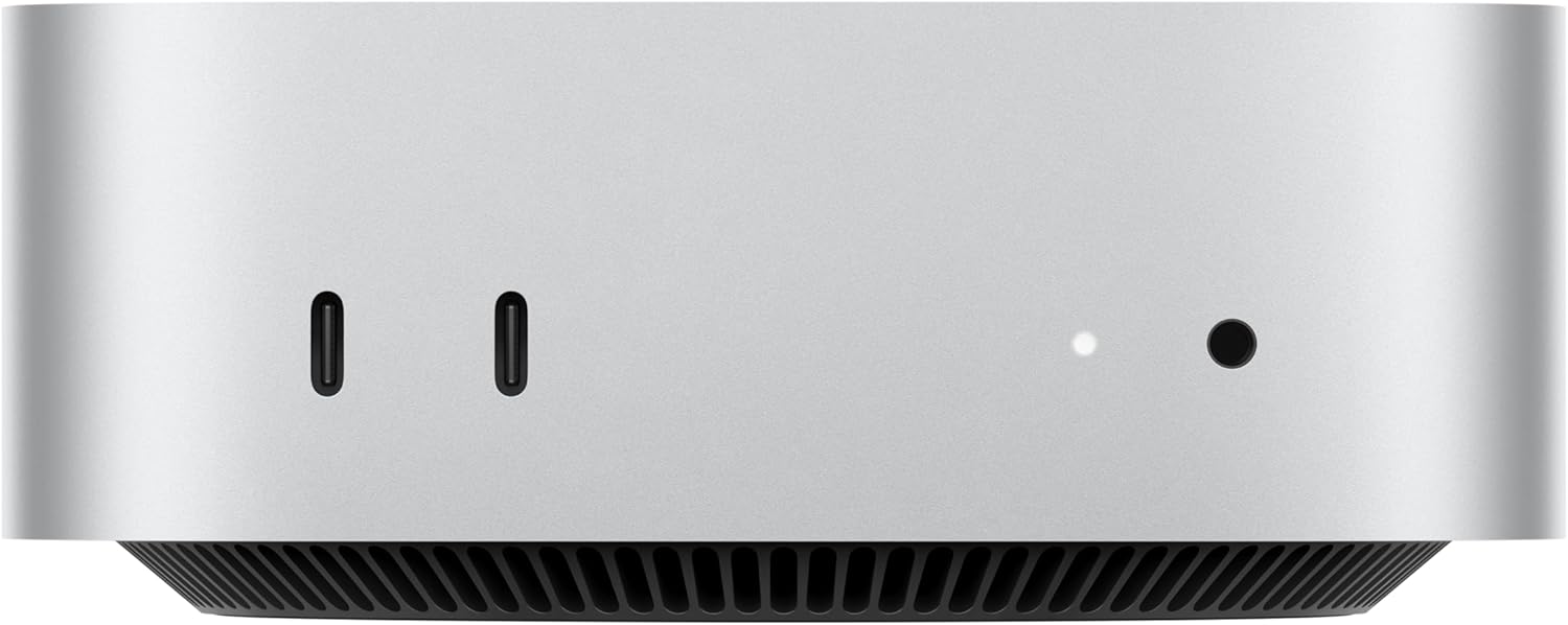
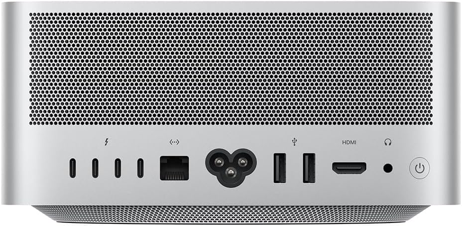
Best Mac for OpenClaw: Mac Mini and Mac Studio Buying Guide
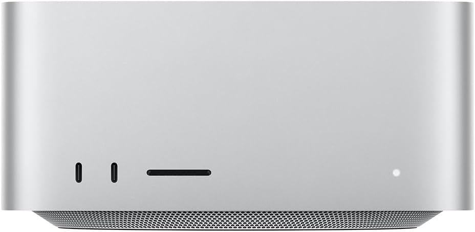
The Mac Mini and Mac Studio have become the go-to hardware for running OpenClaw (formerly Clawdbot). They’re compact, silent, energy efficient, and give you access to macOS-exclusive features like iMessage integration, Voice Wake, and the native menu bar app. But with configurations ranging from a $499 Mac Mini to a $4,000+ Mac Studio, choosing the right one depends entirely on how you plan to use it.
This buying guide breaks down every Mac Mini and Mac Studio configuration that makes sense for OpenClaw, explains which one fits your use case, and includes a comparison table so you can find the right model quickly. If you haven’t decided whether to run OpenClaw locally or in the cloud, our Mac installation guide and DigitalOcean deployment guide cover both options in detail.
How to Think About Mac Mini Specs for OpenClaw
Before looking at specific models, it helps to understand which specs actually matter for running an AI agent like OpenClaw.
RAM is the most important spec. OpenClaw itself is lightweight — it runs on Node.js and doesn’t need much memory for the core gateway and messaging integrations. However, if you also want to run local AI models through Ollama (so you don’t have to pay for cloud API calls), RAM becomes critical. The model must fit entirely in memory to run. You can’t upgrade RAM after purchase on any Apple Silicon Mac, so buy the most you can afford.
CPU matters less than you’d think. OpenClaw’s Node.js runtime is primarily single-threaded, and all M4-series chips have strong single-core performance. You won’t notice a meaningful difference between the base M4 and M4 Pro for the OpenClaw gateway itself. The M4 Pro’s extra cores help if you’re running multiple agents, local models, or doing other compute work on the same machine.
Storage is flexible. OpenClaw’s workspace, configuration files, and memory logs don’t take up much space. The 256GB base model is fine for a dedicated OpenClaw machine. If you’re also running local AI models, those model files can be large (7–70GB each), so 512GB or 1TB gives you more room. External storage via Thunderbolt is always an option for expansion.
Memory bandwidth affects local model speed. If you plan to run local LLMs via Ollama, memory bandwidth directly determines how fast the model generates tokens. The M4 delivers ~120 GB/s, the M4 Pro ~273 GB/s, and the M4 Max ~410–546 GB/s depending on configuration. The M3 Ultra in the Mac Studio reaches ~819 GB/s. For cloud-only API usage, this doesn’t matter much — but for local inference, faster bandwidth means noticeably snappier responses.
Mac Mini and Mac Studio Comparison Table for OpenClaw
Below are the most relevant configurations for running OpenClaw, spanning both the Mac Mini and Mac Studio lineups. Prices listed are Apple MSRP — Amazon frequently discounts these by $50–$100. The “Amazon Link” column is where you can insert your affiliate links.
| Model | Chip | CPU / GPU | RAM | Storage | MSRP | Best For | Amazon Link |
|---|---|---|---|---|---|---|---|
| Mac Mini M4 — Base | M4 | 10-core / 10-core | 16GB | 256GB | $499 | OpenClaw only (cloud AI models) | View on Amazon |
| Mac Mini M4 — 512GB | M4 | 10-core / 10-core | 16GB | 512GB | $599 | OpenClaw + comfortable storage | View on Amazon |
| Mac Mini M4 — 24GB | M4 | 10-core / 10-core | 24GB | 512GB | $799 | OpenClaw + small local models (7B) | View on Amazon |
| Mac Mini M4 Pro — Base | M4 Pro | 12-core / 16-core | 24GB | 512GB | $1,399 | Power users, faster local models | View on Amazon |
| Mac Mini M4 Pro — 48GB | M4 Pro | 12-core / 16-core | 48GB | 512GB | $1,799 | Running 70B local models comfortably | View on Amazon |
| Mac Mini M4 Pro — 48GB / 1TB | M4 Pro | 12-core / 16-core | 48GB | 1TB | $1,999 | Best all-around for serious local AI | View on Amazon |
| Mac Mini M4 Pro — 64GB | M4 Pro | 14-core / 20-core | 64GB | 1TB | $2,399 | Multiple large models, heavy multitasking | View on Amazon |
| Mac Studio (2025) | |||||||
| Mac Studio M4 Max — Base | M4 Max | 14-core / 32-core | 36GB | 512GB | $1,999 | Fast local models, pro multitasking | View on Amazon |
| Mac Studio M4 Max — 64GB | M4 Max | 14-core / 32-core | 64GB | 1TB | $2,599 | Large models with fastest token speed | View on Amazon |
| Mac Studio M4 Max — 16-core / 128GB | M4 Max | 16-core / 40-core | 128GB | 1TB | $3,699 | Frontier models, multi-agent AI lab | View on Amazon |
| Mac Studio M3 Ultra — Base | M3 Ultra | 28-core / 60-core | 96GB | 1TB | $3,999 | 100B+ models, maximum throughput | View on Amazon |
| Mac Studio M3 Ultra — 256GB | M3 Ultra | 32-core / 80-core | 256GB | 2TB | $6,299 | Running the largest open-source models unquantized | View on Amazon |
Note: Some configurations (24GB M4, 48GB M4 Pro, 64GB M4 Pro, and most Mac Studio upgrades) are build-to-order and may only be available directly from Apple.com. Amazon carries the standard base configurations. Check both Amazon and Apple for availability. The Mac Studio M3 Ultra uses the previous-generation M3 chip — Apple has not released an M4 Ultra as of early 2026.
Our Recommendations by Use Case
Best Budget Pick: Mac Mini M4 — 16GB / 512GB ($599)
If you’re using OpenClaw exclusively with cloud AI models like Claude or GPT-4 (no local models), the base-tier M4 Mac Mini is genuinely all you need. OpenClaw’s Node.js gateway is lightweight, and 16GB of RAM handles the agent plus your messaging integrations without breaking a sweat. We recommend the 512GB storage version over the 256GB simply for comfort — the $100 difference gives you room for skills, logs, and general peace of mind. This is the model most people in the OpenClaw community start with.
This is also the configuration to consider if you already have a separate cloud AI subscription (like Anthropic’s API or a Claude Max plan) and just want a dedicated, always-on machine to run the OpenClaw gateway.
Best Value for Local AI: Mac Mini M4 — 24GB / 512GB ($799)
If you want to experiment with running local AI models through Ollama alongside OpenClaw, stepping up to 24GB of unified memory opens the door to smaller models in the 7B–13B parameter range (like Llama 3 8B or Mistral 7B). These models run entirely on-device with no API costs, giving you a fully private AI assistant.
The tradeoff is that the M4’s memory bandwidth (~120 GB/s) is slower than the M4 Pro, so token generation with local models won’t be as fast. For most personal assistant tasks, this is acceptable — you’re trading speed for savings on API costs. This is a build-to-order configuration, so order through Apple.com.
Best Overall: Mac Mini M4 Pro — 48GB / 1TB ($1,999)
This is the sweet spot that power users in the OpenClaw and local AI community have converged on. 48GB of unified memory lets you comfortably run 70B parameter models like Llama 3.1 70B (quantized), which approach the quality of cloud-hosted models. The M4 Pro’s ~273 GB/s memory bandwidth means you’re getting genuinely usable response speeds — not just loading models, but generating tokens fast enough for a natural conversation.
The 1TB storage gives you room to store multiple model files (which can be 40–70GB each), plus OpenClaw’s workspace and any other tools you want to run. The 12-core CPU handles multi-agent setups and background tasks without bogging down. If you can afford it and plan to take local AI seriously, this is the one to buy.
Best for Maximum Capability: Mac Mini M4 Pro — 64GB / 1TB ($2,399)
The 64GB configuration is for users who want to run the largest open-source models at higher quantization levels (Q6/Q8, where output quality is noticeably better), keep multiple models loaded simultaneously, or run multiple OpenClaw agents alongside other memory-intensive work. The upgraded 14-core CPU and 20-core GPU also help if you’re doing any development, rendering, or other compute work on the same machine.
For most people running OpenClaw as a personal assistant, this is overkill. But if you’re building a serious home AI lab or running agents for a team, the extra headroom is worth it.
Should You Buy Used?
Used Mac Minis — especially M1 and M2 models — can be significant bargains. An M2 Pro Mac Mini with 32GB of RAM can be found for around $800–$900 on platforms like Swappa or Back Market, compared to its original price of $1,599+. That’s enough RAM for meaningful local model use at roughly half the cost of a new M4 Pro.
A few things to keep in mind when buying used:
Any Apple Silicon Mac Mini (M1, M2, M4) will run OpenClaw just fine. The M4 is faster, but the M1 and M2 are still very capable for an always-on AI agent using cloud models.
Swappa and Back Market offer buyer protection and verified listings. Facebook Marketplace tends to be 10% cheaper but carries more risk — verify the serial number on Apple’s Check Coverage page before handing over cash.
Always check “About This Mac” on the device to confirm the RAM and storage match the listing. RAM cannot be upgraded after purchase on any Apple Silicon Mac.
When to Choose the Mac Studio Over the Mac Mini
The Mac Studio occupies interesting territory for OpenClaw users. At $1,999, the base M4 Max Mac Studio costs the same as a maxed-out Mac Mini M4 Pro with 48GB and 1TB — but gives you a fundamentally different machine. Here’s how to decide between them.

Mac Studio M4 Max — Base 36GB ($1,999): The Speed Pick
The base Mac Studio gives you the M4 Max chip with ~410 GB/s memory bandwidth — roughly 50% faster than the M4 Pro’s ~273 GB/s. For local AI models, this means significantly faster token generation. If you’re running a 13B–30B parameter model and want the snappiest possible responses, the Mac Studio delivers that at the same price as the top Mac Mini.
The tradeoff: you get 36GB of RAM instead of 48GB. That means slightly smaller models fit comfortably, or you’ll need more aggressive quantization for 70B models. If raw inference speed matters more than fitting the absolute largest models, the base Mac Studio is the pick. It also comes with 10 Gigabit Ethernet (vs. Gigabit on the Mac Mini), an SD card slot, USB-A ports, and four Thunderbolt 5 ports — nice extras for a machine that doubles as a workstation.
Mac Studio M4 Max — 64GB ($2,599): The Sweet Spot for Serious Local AI
Step up to 64GB and you get the best of both worlds — enough RAM for 70B quantized models with room to spare, paired with the M4 Max’s fast memory bandwidth for quick token generation. At $2,599, it’s $200 more than the Mac Mini M4 Pro with 64GB ($2,399), but you’re getting substantially faster inference, more ports, and 10Gb Ethernet. For users who are serious about running large local models as their primary AI backend, this is arguably the best value in the entire lineup.
Mac Studio M4 Max — 128GB ($3,699): The AI Lab
128GB of unified memory opens the door to running frontier-scale open-source models — 100B+ parameter models at reasonable quantization levels, multiple large models loaded simultaneously, or a combination of OpenClaw agents plus development workloads. The upgraded 16-core CPU and 40-core GPU with ~546 GB/s bandwidth make this a genuine AI workstation. This is for users who want to replace cloud API costs entirely with local inference and have the budget to match.
Mac Studio M3 Ultra — 96GB+ ($3,999+): Maximum Everything
The M3 Ultra models are for users who need the absolute maximum memory and throughput. The base M3 Ultra starts at 96GB with ~819 GB/s memory bandwidth — the fastest in the Mac lineup. It’s configurable up to 256GB (and technically up to 512GB through Apple), which means you can run virtually any open-source model at full precision.
One important note: the M3 Ultra uses the previous-generation M3 chip, not the M4. Apple hasn’t released an M4 Ultra as of early 2026 — it may arrive later in the year. For single-threaded performance (which OpenClaw’s Node.js runtime relies on), the M4 Max actually edges out the M3 Ultra. The Ultra wins on multi-core throughput, GPU performance, and raw memory capacity. If you need 96GB+ of RAM right now, the M3 Ultra is your only option in the Mac Studio form factor.
Mac Mini vs. Mac Studio: Quick Decision Framework
Choose the Mac Mini if: You’re using cloud AI models primarily, you want the lowest entry price, or you need up to 64GB of RAM. The Mac Mini M4 Pro with 48GB ($1,999) remains the most popular choice in the OpenClaw community for good reason — it handles the vast majority of use cases at a reasonable price.
Choose the Mac Studio if: Local model inference speed is a priority, you need more than 64GB of RAM, you want 10Gb Ethernet and extra ports, or the machine will double as a workstation for professional creative work. The Mac Studio’s M4 Max delivers meaningfully faster local inference than the M4 Pro at similar price points.
Accessories You’ll Need
Neither the Mac Mini nor the Mac Studio includes a display, keyboard, or mouse. For a dedicated OpenClaw server that you’ll manage remotely, you technically don’t need any of these after initial setup — just plug it into your router via Ethernet, set it up with a borrowed monitor and keyboard, then manage it via SSH and Tailscale going forward.
If you do want a permanent display, any monitor with HDMI or USB-C input works. For initial setup, you can use a TV as a temporary display.
An Ethernet connection is recommended over Wi-Fi for an always-on server. The Mac Mini includes Gigabit Ethernet, while the Mac Studio comes with 10 Gigabit Ethernet — both are built in, so just plug in a cable.
Getting Started After Purchase
Once your Mac Mini or Mac Studio arrives, head over to our complete macOS installation guide for step-by-step setup instructions — including expanded Mac Mini-specific configuration tips for running OpenClaw as a dedicated always-on server. The installation process is identical on both machines.
For ideas on what to automate once it’s running, check out 10 practical things you can do with OpenClaw. And before you give your AI agent broad system access, make sure you’ve read our OpenClaw security guide.
Related Guides on Code Boost
What Is OpenClaw (Formerly Clawdbot)? The Self-Hosted AI Assistant Explained
How to Install OpenClaw on Mac (macOS Setup Guide)
How to Install OpenClaw on Windows (Step-by-Step WSL2 Guide)
How to Install OpenClaw on DigitalOcean (Cloud VPS Guide)
How To Get React to Fetch Data From an API
TL;DR: There are four main ways to fetch data in React: the native Fetch API with useEffect, Axios for more feature-rich HTTP requests, TanStack Query (formerly React Query) for declarative server-state management, and React Server Components for server-side fetching in frameworks like Next.js. Which you reach for depends on your project’s complexity, framework, and whether data lives on the client or server.
Fetching data from an API is one of the most common tasks in React development. React doesn’t prescribe a specific approach — it leaves the choice to you — which means there are several valid patterns, each with different trade-offs. This guide covers all of them with accurate, up-to-date code examples so you can choose the right tool for your use case.
The Four Main Approaches
Before diving in, here’s a quick orientation of when to use each method:
- Fetch API + useEffect — Simple, no dependencies, good for straightforward client-side fetching in smaller apps or isolated components.
- Axios + useEffect — Like Fetch but with a cleaner API, automatic JSON parsing, and better interceptor support. Good for apps already using Axios.
- TanStack Query (useQuery) — The go-to for client-side data in real-world apps. Handles caching, background refetching, deduplication, and loading/error states automatically.
- React Server Components — The modern framework-native approach for Next.js 13+ and other RSC-enabled frameworks. Fetches data on the server with zero client-side JavaScript overhead.
1. The Native Fetch API with useEffect
The Fetch API is built into the browser — no libraries needed. Combined with useEffect and useState, it’s the most lightweight way to fetch data in a React component.
import { useState, useEffect } from 'react';

function UserList() {
  const [data, setData] = useState(null);
  const [loading, setLoading] = useState(true);
  const [error, setError] = useState(null);

  useEffect(() => {
    const controller = new AbortController();

    fetch('https://api.example.com/users', { signal: controller.signal })
      .then(response => {
        if (!response.ok) throw new Error('Network response was not ok');
        return response.json();
      })
      .then(data => {
        setData(data);
        setLoading(false);
      })
      .catch(err => {
        if (err.name !== 'AbortError') {
          setError(err.message);
          setLoading(false);
        }
      });

    return () => controller.abort();
  }, []);

  if (loading) return <p>Loading...</p>;
  if (error) return <p>Error: {error}</p>;
  return <ul>{data.map(user => <li key={user.id}>{user.name}</li>)}</ul>;
}
A few things worth noting in this example that are often skipped in basic tutorials:
- AbortController — The cleanup function calls
controller.abort()when the component unmounts, cancelling the in-flight request and preventing state updates on unmounted components (a common source of memory leak warnings). - Response.ok check — Fetch doesn’t throw on HTTP error status codes (like 404 or 500). You need to check
response.okmanually and throw if needed. - Separate loading and error states — Essential for a good user experience.
When to use it: Simple components or small apps where adding a library feels like overkill. If you’re writing the same loading/error boilerplate in five places, it’s time to move to TanStack Query.
2. Axios: A Cleaner HTTP Client
Axios is a popular third-party HTTP library that improves on the native Fetch API in several ways: it throws automatically on non-2xx status codes, parses JSON responses by default, supports request/response interceptors for auth headers and logging, and has cleaner timeout handling.
Install it first:
npm install axiosThen use it with useEffect:
import { useState, useEffect } from 'react';
import axios from 'axios';

function UserList() {
  const [data, setData] = useState(null);
  const [loading, setLoading] = useState(true);
  const [error, setError] = useState(null);

  useEffect(() => {
    const controller = new AbortController();

    axios.get('https://api.example.com/users', { signal: controller.signal })
      .then(response => {
        setData(response.data);
        setLoading(false);
      })
      .catch(err => {
        if (!axios.isCancel(err)) {
          setError(err.message);
          setLoading(false);
        }
      });

    return () => controller.abort();
  }, []);

  if (loading) return <p>Loading...</p>;
  if (error) return <p>Error: {error}</p>;
  return <ul>{data.map(user => <li key={user.id}>{user.name}</li>)}</ul>;
}
Axios also works well with async/await for cleaner sequential logic:
useEffect(() => {
  const controller = new AbortController();

  const fetchData = async () => {
    try {
      const response = await axios.get('https://api.example.com/users', {
        signal: controller.signal
      });
      setData(response.data);
    } catch (err) {
      if (!axios.isCancel(err)) setError(err.message);
    } finally {
      setLoading(false);
    }
  };

  fetchData();
  return () => controller.abort();
}, []);
When to use it: Projects that need interceptors (attaching auth tokens to every request, for example), centralized error handling, or that already have Axios configured as a base instance across the codebase.
3. TanStack Query (Formerly React Query)
TanStack Query is the most widely adopted solution for managing server state in React. It treats data fetched from APIs as a distinct concern from UI state — handling caching, background refetching, request deduplication, stale-while-revalidate patterns, and loading/error states automatically, so you don’t have to.
Note: “React Query” was renamed to TanStack Query when it expanded to support other frameworks. The React package is @tanstack/react-query.
Install it:
npm install @tanstack/react-queryWrap your app in the provider (typically in your root component):
import { QueryClient, QueryClientProvider } from '@tanstack/react-query';

const queryClient = new QueryClient();

export default function App() {
  return (
    <QueryClientProvider client={queryClient}>
      <UserList />
    </QueryClientProvider>
  );
}
Then use useQuery in your components — note the current v5 API uses an options object, not a positional string key:
import { useQuery } from '@tanstack/react-query';

async function fetchUsers() {
  const response = await fetch('https://api.example.com/users');
  if (!response.ok) throw new Error('Failed to fetch');
  return response.json();
}

function UserList() {
  const { data, error, isPending } = useQuery({
    queryKey: ['users'],
    queryFn: fetchUsers,
  });

  if (isPending) return <p>Loading...</p>;
  if (error) return <p>Error: {error.message}</p>;
  return <ul>{data.map(user => <li key={user.id}>{user.name}</li>)}</ul>;
}
What TanStack Query handles for you automatically that plain useEffect doesn’t:
- Caching — The same query across multiple components only fires one network request. Subsequent renders use cached data instantly.
- Background refetching — When a user returns to a tab or reconnects to the network, stale data is quietly refreshed in the background.
- Request deduplication — Multiple components mounting simultaneously won’t fire duplicate requests for the same data.
- Automatic retries — Failed requests are retried automatically (configurable).
- Mutations — The
useMutationhook handles POST/PUT/DELETE operations with optimistic update support and cache invalidation.
When to use it: Any real-world app where data is shared across components, needs to stay fresh, or where writing loading/error boilerplate in every component is becoming a burden. For most production React apps, TanStack Query is the right default for client-side data fetching.
4. React Server Components
React Server Components (RSC) represent a fundamentally different approach to data fetching — instead of fetching data on the client after the component renders, the component fetches its data on the server before sending any HTML to the browser. This eliminates client-side loading spinners for the initial data load, reduces JavaScript bundle size, and avoids request waterfalls on the client.
In Next.js 13+ with the App Router, all components are Server Components by default. Fetching data is as simple as making a component async:
// app/users/page.tsx — Server Component (no 'use client' directive)
async function UserList() {
  const response = await fetch('https://api.example.com/users', {
    next: { revalidate: 60 } // revalidate every 60 seconds
  });
  const users = await response.json();

  return (
    <ul>
      {users.map(user => (
        <li key={user.id}>{user.name}</li>
      ))}
    </ul>
  );
}
There’s no useEffect, no useState, no loading state management — the data is ready before the component renders. Next.js extends fetch with caching options (force-cache, no-store, revalidate) to give you fine-grained control over freshness.
For highly interactive components that still need client-side data (real-time updates, user-triggered refetches), the recommended pattern in modern Next.js apps is to combine Server Components for the initial load with TanStack Query for client-side updates — giving you the best of both.
When to use it: Framework-based React apps using Next.js 13+ App Router (or TanStack Start, Remix). Not available in plain Create React App or Vite setups without a framework layer.
Best Practices for Fetching Data in React
Always handle errors explicitly. Fetch doesn’t throw on 4xx/5xx responses — check response.ok and throw manually. TanStack Query propagates thrown errors through its error state automatically.
Cancel requests on unmount. Use AbortController with a cleanup function in useEffect to cancel in-flight requests when a component unmounts. This prevents “can’t perform a state update on an unmounted component” warnings.
Show meaningful loading states. Avoid blank screens — display skeletons or spinners while data loads. TanStack Query’s isPending and isFetching flags make this easy to distinguish between “no data yet” and “refreshing in the background.”
Use query keys thoughtfully. In TanStack Query, query keys are the cache identity for your data. Include any variables the query depends on — ['users', userId] rather than just ['users'] — so the cache is correctly invalidated when parameters change.
Don’t fetch in useEffect when a framework can do it for you. If you’re using Next.js, Remix, or TanStack Start, reaching for Server Components or loader functions is often cleaner and more performant than client-side useEffect fetching for initial page data.
Cache deliberately. Both TanStack Query’s staleTime/gcTime settings and Next.js’s fetch cache options give you control over how long data stays fresh. Set these based on how frequently your data actually changes — aggressive caching can significantly improve perceived performance.
Choosing the Right Approach
| Scenario | Recommended Approach |
|---|---|
| Simple component, no framework | Fetch API + useEffect + AbortController |
| Need interceptors or centralized HTTP config | Axios + useEffect |
| Data shared across components / needs caching | TanStack Query |
| Mutations with cache invalidation | TanStack Query (useMutation) |
| Next.js App Router / RSC-enabled framework | React Server Components (+ TanStack Query for interactive parts) |
| Real-time data (WebSockets, polling) | TanStack Query with refetchInterval, or dedicated WS library |
Frequently Asked Questions
Is it bad to fetch data in useEffect?
Not inherently — it’s a valid pattern for simple cases. The problem is that raw useEffect data fetching doesn’t handle caching, deduplication, or background refetching, so it tends to accumulate boilerplate as apps grow. For anything beyond a single component fetching its own isolated data, TanStack Query is a better fit.
What’s the difference between React Query and TanStack Query?
They’re the same library. React Query was renamed TanStack Query when the project expanded support beyond React to Vue, Solid, and other frameworks. The React-specific package is @tanstack/react-query and the API is the same.
Should I use the v3 or v5 API for TanStack Query?
Use v5. The old positional string key syntax — useQuery('key', fn) — was deprecated in v4 and removed in v5. The current API uses an options object: useQuery({ queryKey: ['key'], queryFn: fn }). Also note that isLoading was renamed to isPending in v5.
Do React Server Components replace TanStack Query?
For initial data loads in framework-based apps, yes — Server Components are often cleaner. But TanStack Query still handles use cases that RSC doesn’t: client-side mutations, optimistic updates, polling, infinite scroll, and any data that needs to stay live after the initial page load. The hybrid pattern (RSC for initial render, TanStack Query for interactivity) has become the dominant approach in Next.js apps.
How do I handle authentication headers when fetching data?
With Axios, set up a base instance with default headers. With Fetch or TanStack Query, create a wrapper function that adds your auth header before calling fetch. TanStack Query doesn’t manage HTTP configuration directly — it calls whatever queryFn you provide, so auth handling lives in that function.
For a deeper look at how React handles state alongside data, see our guide on React Hooks basics including useState and useEffect. If you’re using Next.js as your React framework, our Next.js basics guide covers the server-rendering fundamentals that underpin React Server Components.
AI Models Don’t “Think.” They Predict.
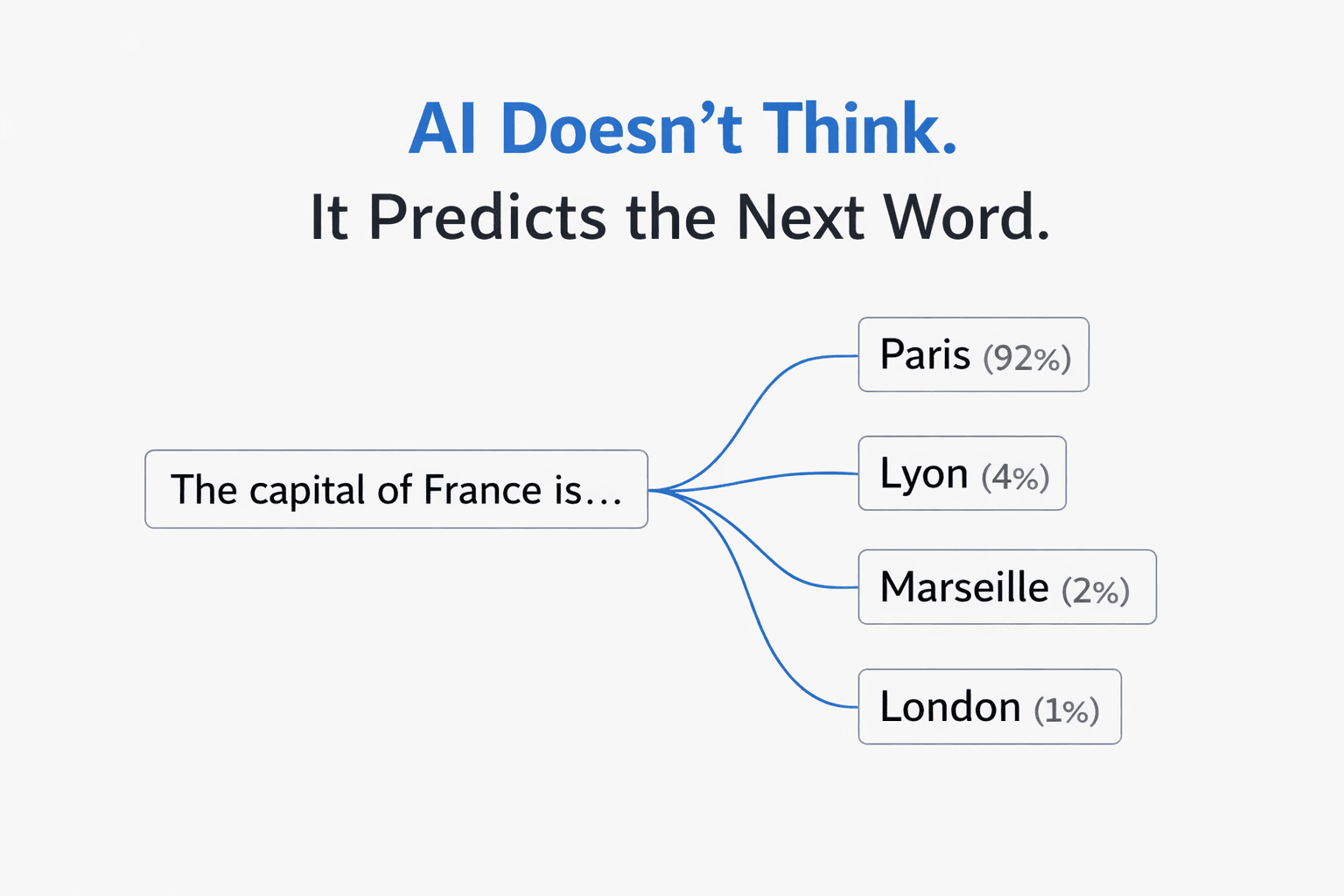
AI Models Don’t “Think.” They Predict.
The single most important thing to understand: a large language model is a prediction engine. It reads your entire prompt, then predicts the next word (technically, the next “token”) based on statistical patterns from its training data. Then it predicts the next word after that. And the next. One at a time, until it builds a full response.
It does not plan ahead. It does not understand your intent. It does not “know” anything. It recognizes patterns and predicts what text is most likely to follow the text you gave it.
This has a profound implication: the quality of the prediction is entirely determined by the quality of the input. Better input patterns produce better output patterns. That’s the whole game.
Every effective prompting technique — including KERNEL — works because it gives the prediction engine a higher-quality input pattern to work from.
Why “Simple” Is the Wrong Frame
The KERNEL framework starts with “Keep it simple” — suggesting that shorter prompts with less context produce better results. And for basic code tasks, that’s often true.
But the underlying principle isn’t simplicity. It’s signal-to-noise ratio.
Language models use something called an attention mechanism — a system that decides which parts of your prompt to focus on when generating each word. When your prompt is full of irrelevant context, the attention mechanism gets diluted. The model pays attention to everything equally, including the noise, and the output quality degrades.
This is why a 500-word prompt full of background rambling produces worse results than a 50-word focused prompt. But it’s also why a 500-word prompt that’s well-structured — with clear sections, labeled data, and the task at the end — can dramatically outperform the short version for complex tasks.
The “Lost in the Middle” Problem
There’s a well-documented phenomenon in language model research: performance drops by up to 30% when critical information is placed in the middle of a long prompt, compared to placing it at the beginning or the end.
The model’s attention is strongest at the start and end of your input. The middle gets less focus — it’s the cognitive equivalent of someone’s eyes glazing over during a long meeting.
This explains why the KERNEL framework’s “Logical structure” rule works so well. When you put your context first and your task last, you’re placing information exactly where the attention mechanism is strongest:
| Position | What to Place Here | Why |
|---|---|---|
| Beginning | Background data, documents, context | Strong attention. Gets processed and retained. |
| Middle | Examples, rules, formatting guidance | Weakest attention. Keep this structured and labeled. |
| End (last line) | Your specific task or question | Strongest attention. The model generates its response from here. |
This is the theoretical basis for why structured prompt frameworks (like the Bento-Box method) consistently outperform unstructured prompts — even when they contain the same information.
Why Positive Instructions Beat Negative Constraints
The KERNEL framework recommends telling AI “what NOT to do.” This is one area where the empirical advice conflicts with the research.
Both Anthropic and OpenAI’s documentation specifically recommend positive framing over negative constraints. Here’s why it matters at the model level:
When you write “don’t use external libraries,” the model has to process the concept of external libraries, recognize it as something to avoid, and then navigate around it. But the prediction engine doesn’t have a clean “avoidance” mechanism — it processes the concept either way, and the mere presence of “external libraries” in the prompt can increase the probability of those tokens appearing in the output.
❌ Negative framing
“No external libraries. No functions over 20 lines. Don’t use global variables.”
✅ Positive framing
“Use only Python standard library. Keep each function under 20 lines. Use local variables with descriptive names.”
Same constraints. Different framing. The positive version gives the model a clear target pattern to follow, rather than a pattern to avoid.
Why Examples Work Better Than Descriptions
The KERNEL framework doesn’t explicitly cover few-shot prompting (providing examples), but this is one of the most powerful techniques available — and the theory explains why.
When you describe what you want (“write professional, concise emails”), the model has to interpret those adjectives and map them to a style. That interpretation is fuzzy. “Professional” means different things in different contexts.
When you show what you want (by providing 3–5 examples of the input-output pattern), you’re giving the model a concrete statistical pattern to match. It doesn’t have to interpret anything — it just extends the pattern you’ve established.
The Temperature Variable Most People Miss
Every prompt framework focuses on the words you write — but there’s a hidden variable most people never adjust: temperature.
Temperature controls how the model navigates its probability list when choosing each word. At temperature 0.0, it always picks the highest-probability word (deterministic, consistent, factual). At temperature 1.0, it samples more broadly from the distribution (creative, varied, surprising).
This is why the same prompt can produce wildly different results on different days — and why KERNEL’s “Reproducible results” principle is harder to achieve than it sounds. If you’re using a web chat interface, the temperature is set for you by the platform. But if you have access to settings or are using an API, matching the temperature to the task type is one of the highest-leverage adjustments you can make.
| Task Type | Ideal Temperature | Why |
|---|---|---|
| Code, math, data extraction | 0.0 – 0.2 | One correct answer. No creativity needed. |
| Business writing, emails | 0.5 – 0.7 | Professional but not robotic. |
| Brainstorming, creative writing | 0.8 – 1.0 | Many possible good answers. Variety is the goal. |
Where Frameworks Like KERNEL Fall Short
To be clear: KERNEL is a good framework. If you’re a developer writing code prompts, following it will improve your results significantly.
But it has three limitations worth noting:
1. It’s code-focused. The examples are all about scripts and data processing. Most people using AI aren’t writing code — they’re writing emails, creating content, analyzing data, learning new topics, making decisions. The principles are similar, but the application looks very different.
2. It doesn’t cover multi-turn interaction. One of the most powerful prompting techniques available in web chat interfaces is using follow-up messages to iteratively refine output. Most beginners treat their first prompt as the final product. In practice, the conversation is the prompt.
3. It’s model-agnostic by design — but models aren’t interchangeable. Claude handles XML-structured prompts better than any other model. GPT’s Structured Outputs can guarantee 100% JSON schema compliance. Gemini can process 2 million tokens of context at once. Knowing these model-specific strengths lets you choose the right tool for the job.
The Practical Version
Understanding why prompts work is useful. But what most people actually need is a set of practical, actionable best practices they can apply immediately — across any model, any task, any experience level.
I put together a comprehensive breakdown of the techniques that consistently produce better AI output, with before/after examples, decision frameworks, and ready-to-use patterns:
→ AI Prompt Engineering Best Practices: The Complete Guide
It covers the 5-Part Prompt Formula, the three core techniques (Zero-Shot, Few-Shot, Chain-of-Thought), when to use each one, the most common mistakes, and model-specific tips for ChatGPT, Claude, and Gemini.
If you found the theoretical breakdown here useful, that post is the practical playbook.
AI Prompt Engineering Best Practices

Want The Full Guide?
AI prompt engineering best practices aren’t about memorizing magic phrases or gaming the system. They’re a set of simple, repeatable principles that help you get dramatically better results from any AI tool — whether you use ChatGPT, Claude, Gemini, Copilot, or anything else.
The problem? Most people are still prompting the way they did in 2023. Short, vague requests. No structure. No context. And they’re wondering why the AI keeps giving them generic, surface-level answers.
This guide breaks down exactly what works in 2026 — from foundational concepts to advanced techniques — so you can stop guessing and start getting output that’s actually useful.
What Is Prompt Engineering (And Why Should You Care)?
Prompt engineering is the process of designing clear, structured inputs that guide an AI model toward accurate, useful output. That’s it. No computer science degree required.
Here’s why it matters: the quality of what you get from AI is almost entirely determined by the quality of what you put in. The model’s intelligence isn’t the bottleneck — your instructions are.
Think of AI as a brilliant new hire. They’ve read every book and article ever written, but they know absolutely nothing about your specific project, your preferences, or your audience. If you tell that new hire “fix the code,” they’ll fail. If you tell them “Review this Python 3.11 function for bugs. It should accept a list of integers and return the sum of even numbers only. Follow PEP 8 conventions” — now they can deliver.
That gap between vague and specific is the entire game of prompt engineering.
The 7 AI Prompt Engineering Best Practices That Actually Work
These aren’t theoretical. These are the principles that consistently produce better output across every major AI model.
1. Be Specific — Ruthlessly Specific
The #1 reason people get bad AI output is vagueness. Every detail you leave out is a detail the AI has to guess — and it will guess wrong.
❌ Weak Prompt“Write me a blog post about marketing.”
✅ Strong Prompt“Write an 800-word blog post about email marketing strategies for e-commerce stores with under $50K/month in revenue. Target audience: solo founders. Tone: practical and conversational. Include 3 actionable tips with real-world examples.”
The strong prompt specifies the topic, length, audience, tone, structure, and what “good” looks like. The AI doesn’t have to guess any of it.
2. Assign a Role
Starting your prompt with “You are a…” is one of the simplest and most effective upgrades you can make. It frames the entire response through a specific lens of expertise.
- Need a workout plan? → “You are a certified personal trainer.”
- Writing a cover letter? → “You are a hiring manager at a Fortune 500 company.”
- Explaining something complex? → “You are a patient middle school teacher.”
- Debugging code? → “You are a senior Python developer doing a code review.”
This single line changes the vocabulary, depth, and perspective of the entire response.
3. Tell the AI What TO Do, Not What NOT to Do
This is one of the most well-documented findings in prompt engineering research: AI models respond much better to positive instructions than negative constraints.
❌ Negative Framing“Don’t use jargon. Don’t make it too long. Don’t include irrelevant details.”
✅ Positive Framing“Use simple, everyday language. Keep the response under 200 words. Focus only on the three main benefits.”
Negative instructions can actually increase the chance the AI does the thing you’re trying to prevent. Positive framing gives it a clear target to aim for.
4. Use the 5-Part Prompt Formula
For any important prompt, run through this checklist:
| # | Component | What It Does | Example |
|---|---|---|---|
| 1 | Role | Tells the AI who to be | “You are an experienced email copywriter.” |
| 2 | Context | Background the AI needs | “Our company sells eco-friendly products to women 25–40.” |
| 3 | Task | Exactly what you want done | “Write 5 email subject lines for our spring sale.” |
| 4 | Format | Shape of the output | “Keep each under 50 characters.” |
| 5 | Constraints | Rules or boundaries | “No clickbait. No ALL CAPS.” |
You don’t need all five for simple questions. But when the AI keeps giving you something generic or off-target, check which component you’re missing — that’s usually the fix.
5. Show Examples (Few-Shot Prompting)
If you need the output in a very specific format, tone, or style, the most effective technique is to show the AI what good looks like. This is called few-shot prompting, and 3–5 examples is the sweet spot.
✅ Few-Shot ExampleClassify these customer messages by sentiment:
Input: “Love this product! Best purchase ever.” → Output: Positive
Input: “Arrived broken. Very disappointed.” → Output: Negative
Input: “It’s okay, nothing special.” → Output: Neutral
Now classify this:
Input: “Shipping was slow but the quality is great.”
The AI learns the pattern from your examples and applies it consistently. This is especially powerful for classification, formatting, and maintaining a consistent brand voice.
6. Make the AI Show Its Work (Chain-of-Thought)
For any task involving math, logic, analysis, or multi-step reasoning, adding one simple phrase dramatically improves accuracy: “Let’s think step by step.”
This forces the AI to generate intermediate reasoning steps instead of jumping straight to an answer — and each step gives the next step better context. It’s called Chain-of-Thought prompting, and it’s one of the most well-researched techniques in the field.
For even better results, you can tell the AI exactly what steps to follow:
1. Describe what the code is supposed to do.
2. Walk through the logic line by line.
3. Identify edge cases that aren’t handled.
4. List each bug with the line number.
5. Provide the corrected code.”
Heads up: Chain-of-Thought generates more text (the reasoning steps), which means it uses more tokens and is slightly slower. Use it when accuracy matters — not for simple questions where a direct answer works fine.
7. Use Follow-Up Messages to Refine
This is the technique most beginners miss entirely: the conversation itself is a prompt engineering tool.
You don’t have to nail everything in one message. The AI remembers the full conversation, so you can start broad and refine:
| Message | What You Say |
|---|---|
| 1st | “Write a product description for a stainless steel water bottle.” |
| 2nd | “Make it more casual and fun. Target audience is college students.” |
| 3rd | “Add a line about the lifetime warranty. Keep it under 80 words.” |
| 4th | “Perfect. Now give me 3 variations for A/B testing.” |
Each follow-up builds on the full context of the conversation. This “refine as you go” approach is often easier and more effective than trying to write the perfect prompt on the first try.
Quick Reference: Technique Comparison
Different tasks call for different techniques. Here’s how to choose:
| Technique | What It Is | When to Use It |
|---|---|---|
| Zero-Shot | Direct instruction, no examples | Simple questions, translations, summaries |
| Few-Shot | Providing 3–5 example pairs | Specific formats, classification, consistent tone |
| Chain-of-Thought | Forcing step-by-step reasoning | Math, logic, debugging, multi-step analysis |
| Role Prompting | Assigning a persona (“You are a…”) | Any task where expertise or perspective matters |
| Step-Back | Ask a general question first, then the specific one | Creative tasks where the AI gives shallow answers |
The Biggest Mistakes People Make
After analyzing hundreds of prompts, these are the patterns that consistently produce bad output:
- Being too vague. “Help me with marketing” gives the AI nothing to work with. Be specific about what, for whom, and in what format.
- Not providing context. The AI doesn’t know your business, your audience, or your goals unless you tell it.
- Accepting the first response as final. The first output is a draft. Use follow-ups to shape it into exactly what you need.
- Dumping a document with no instructions. Pasting 5,000 words and hoping for the best doesn’t work. Tell the AI what to do with it.
- Asking multiple unrelated questions in one prompt. Ask one thing at a time, or number your questions clearly.
- Never specifying the audience. “Explain this” is ambiguous. “Explain this for a non-technical executive” is actionable.
These Principles Work Across Every AI Model
Whether you’re using ChatGPT, Claude, Gemini, Copilot, or any other tool — these best practices work because they’re based on how language models process information, not on any platform-specific trick.
That said, each model does have specific strengths worth knowing about:
- Claude excels with XML-structured prompts and handles complex, multi-part instructions particularly well.
- ChatGPT (GPT-4/5) has strong system message persistence and offers Structured Outputs for guaranteed JSON formatting.
- Gemini can process massive context windows (up to 2 million tokens) and handles multimodal input (text + images + video).
The fundamentals — clarity, specificity, structure, examples, and iteration — are universal.
Want the Complete System? Get the Full Guide Pack.
AI Prompt Engineering Best Practices — The Complete Bundle
Everything in this article (and a whole lot more) organized into 6 step-by-step guides, a 37-prompt template library, and a quickstart welcome sheet.
| ✅ Guide 1: How AI Actually Works (the mental model) |
| ✅ Guide 2: Structuring Prompts (Delimiters & Bento-Box) |
| ✅ Guide 3: Core Techniques (Zero-Shot, Few-Shot, CoT) |
| ✅ Guide 4: Tuning Knobs (Temperature, Top-P, Top-K) |
| ✅ Guide 5: Advanced Strategies & Model-Specific Tips |
| ✅ Guide 6: Practical Prompting for Web Chat Users |
| ✅ Prompt Library: 37 Copy-Paste Templates |
| ✅ Welcome Quickstart Sheet |
Google Docs–compatible .docx files. Instant download. No coding or API access required.
Start Improving Your Prompts Today
You don’t need to master everything at once. Start with the two highest-impact changes:
- Be specific. Add context, audience, format, and constraints to your next prompt and compare the result to what you normally get.
- Use follow-ups. Stop treating your first prompt as final. Send it, then refine with 2–3 follow-up messages.
That alone will put you ahead of the vast majority of AI users. And if you want the full system — the complete guides, ready-to-use templates, model-specific strategies, and advanced techniques — grab the complete bundle here.
The models keep getting smarter. But the gap between a careless prompt and a well-engineered one isn’t closing — it’s widening. The people who learn this skill now will compound that advantage every single day they use AI.
Want the complete system with 6 guides, 37 prompt templates, and model-specific cheat sheets? Get the AI Prompt Engineering Best Practices bundle →
How to Install OpenClaw with Docker (Step-by-Step)
What This Guide Covers
This guide walks through installing OpenClaw using Docker, the easiest and most reliable way to run it locally.
By the end of this guide you’ll have:
-
OpenClaw running in a Docker container
-
The gateway configured
-
Your first agent ready to connect to AI providers
This method works on:
-
macOS
-
Linux
-
Windows (WSL2)
-
Synology / NAS environments that support Docker
What OpenClaw Actually Installs
Before installing, it helps to understand what you’re running.
OpenClaw consists of three main pieces:
| Component | What it does |
|---|---|
| Gateway | The core service that runs the agent |
| Workspace | The environment where the agent performs tasks |
| AI Provider | The model powering the agent (OpenAI, Anthropic, etc.) |
Docker packages these pieces into a container so you don’t need to manually install dependencies.
Requirements
Before installing OpenClaw you need:
1. Docker installed
Check if Docker is installed:
If it isn’t installed yet:
-
macOS / Windows → Install Docker Desktop
-
Linux → Install Docker Engine
Minimum recommended system:
| Resource | Recommendation |
|---|---|
| RAM | 8GB |
| CPU | 4 cores |
| Disk | 10GB free |
OpenClaw can run on less, but builds may take longer.
Step 1 — Clone the OpenClaw Repository
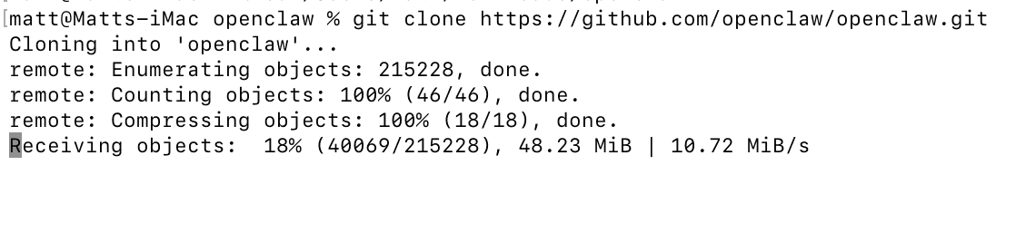
Download the project from GitHub.
cd openclaw
This repository includes:
-
Docker configuration
-
setup scripts
-
onboarding tools
-
environment configuration
Step 2 — Run the Docker Setup Script
The easiest way to install OpenClaw is using the included setup script.
This script automatically:
-
Builds or pulls the OpenClaw Docker image
-
Starts the Docker containers
-
Runs onboarding
-
Creates the
.envconfiguration file -
Generates your gateway token
You do not need to manually run Docker commands.
Optional: Use the Prebuilt Image (Faster)
If you want to avoid building locally, you can use the official container image.
This can save several minutes during installation.
Step 3 — Complete Onboarding
During setup you’ll be asked to configure your AI provider.
Common choices:
| Provider | Notes |
|---|---|
| OpenAI | Most widely used |
| Anthropic | Often better for reasoning |
| Local models | Possible but requires more setup |
You will typically enter an API key.
Example:
Step 4 — Start the Gateway
Once setup finishes, start OpenClaw.
This launches the gateway container in the background.
Step 5 — Verify OpenClaw Is Running
Check container status:
You should see something like:
If it is running, the installation succeeded.
You can also check logs:
Where OpenClaw Stores Data
By default OpenClaw stores data inside the container.
For persistent data, you can mount a workspace folder.
Example:
This allows agents to keep files between restarts.
Updating OpenClaw
To update OpenClaw later:
docker compose pull
docker compose up -d
Troubleshooting
Docker build fails
Try using the prebuilt image:
Container stops immediately
Check logs:
Most failures come from:
-
missing API keys
-
incorrect environment variables
-
port conflicts
Out of memory errors
OpenClaw builds can require several gigabytes of RAM.
Try increasing Docker memory limits or using the prebuilt image.
Optional Advanced Setup
Advanced users may want to enable:
-
sandbox mode
-
browser automation
-
persistent workspaces
-
multi-agent orchestration
These require additional Docker configuration.
Final Thoughts
Installing OpenClaw with Docker removes most of the complexity of dependency management. Once running, you can begin experimenting with autonomous agents, automation workflows, and AI-driven tasks.
How Much Does Claude Code Cost? Pricing, Plans, and How to Save Money
Claude Code is available through Anthropic’s subscription plans starting at $20 per month, with higher tiers offering more usage and access to the most powerful models. You can also use pay-as-you-go API billing for more flexibility. This guide breaks down every option so you can choose the plan that matches how you actually work and avoid paying more than you need to.
If you are new to Claude Code, start with our overview of what Claude Code is before diving into pricing. Ready to get started? Head to our installation guide.
Anthropic offers several subscription tiers that include Claude Code. Each uses session-based usage limits that reset every five hours, so your capacity refreshes throughout the day rather than being a single monthly allowance.
The Free plan provides access to Claude.ai chat but very limited Claude Code functionality. For any real development work, a paid plan is necessary.
The Pro plan costs $20 per month billed monthly, or $17 per month with annual billing. It includes Claude Code access with moderate limits, roughly 10 to 40 prompts every five hours depending on complexity. Pro works for learning Claude Code, light development, and occasional coding sessions. It also includes file creation, code execution, Projects, and web search.
The Max plan comes in two tiers. Max 5x at $100 per month gives you five times the Pro usage. Max 20x at $200 per month gives twenty times Pro limits. Both include access to the Opus model, the most capable for complex engineering, and priority during high-demand periods. Max is for developers who rely on Claude Code as a primary daily tool.
API Pay-As-You-Go Pricing
If you prefer usage-based billing, use Claude Code with an Anthropic Console account and API key. You pay per token, with costs varying by model. Sonnet runs $3 per million input tokens and $15 per million output tokens. Opus costs significantly more but delivers stronger reasoning.
API pricing offers precise cost control and no hard usage caps, which matters for automation and scaling. However, costs can be variable and high with heavy use. One developer tracked eight months of heavy daily usage that would have cost over $15,000 on API pricing but only $800 on the Max plan. For most developers using Claude Code daily, the subscription wins on cost.
The API also offers batch processing at 50 percent off for non-urgent tasks and prompt caching that charges only 10 percent for cached content after the first request. System prompts and CLAUDE.md files are cached automatically.
Team and Enterprise Plans
For organizations, the Team plan starts at $25 per Standard seat per month with annual billing. Standard seats include collaboration features but not Claude Code. Premium seats at $150 per month add Claude Code access and early features, suited for technical teams. Enterprise plans include all Team features with additional governance and security. Contact Anthropic for Enterprise pricing.
Which Plan Should You Choose?
If you are starting out or use Claude Code a few times per week, Pro at $20 per month provides enough capacity for learning and light tasks. You will hit limits during sustained sessions, but for occasional use it works.
If Claude Code is a regular part of your workflow, Max 5x at $100 per month is the sweet spot. It handles daily professional work including complex debugging, feature implementation, and code review without constant limit interruptions.
For power users running Claude Code continuously across multiple projects or needing unrestricted Opus access, Max 20x at $200 per month offers the highest capacity. If your equivalent API costs would exceed $200 monthly, this tier saves significant money.
If your usage is unpredictable or you are integrating Claude Code into automated pipelines, API billing provides flexibility but requires monitoring. Start with a small amount of credits to understand your patterns before committing.
How to Track and Reduce Costs
The /cost command shows your session’s token usage and estimated cost, most useful for API users. For continuous visibility, configure the status line to show token usage at all times.
The most effective cost reduction strategies are clearing context between tasks with /clear so you stop paying for irrelevant history, using /compact to summarize long conversations, and choosing Sonnet over Opus for routine tasks. Sonnet handles most coding work well at much lower cost per token.
For teams, administrators set workspace spend limits in the Anthropic Console and view usage reports. The average API cost is roughly $6 per developer per day, with 90 percent of users staying below $12 daily. For configuration details, see our setup guide.
Understanding Usage Limits
Anthropic introduced weekly rate limits in August 2025 on top of the five-hour session resets. These primarily affect power users running Claude Code continuously and impact less than five percent of subscribers according to Anthropic. Pro and Max plans have different thresholds, with Max getting proportionally higher caps.
Claude Code sessions consume more capacity than regular chat because they include system instructions, full file contexts, long code outputs, and multiple tool calls per interaction. You will use your allocation faster than in the Claude.ai chat interface. Max subscribers can purchase additional usage beyond rate limits at standard API rates if needed.
For more on how tokens and context windows work technically, read how Claude Code works under the hood. To learn practical efficiency techniques, see our guide to using Claude Code effectively.
How Does Claude Code Work? Models, Architecture, and MCP Integration Explained
Claude Code is more than a chatbot that writes code. It is an agentic system that reads your files, executes terminal commands, manages git operations, connects to external services, and coordinates with other tools, all while maintaining awareness of your full codebase. Understanding how it works helps you use it more effectively, choose the right model, manage context, and extend it with external tools through MCP.
For a general overview of what Claude Code does, see what is Claude Code. To start using it right away, check out how to use Claude Code.
Claude Code runs on Anthropic’s Claude family of large language models. By default, it uses Claude Sonnet, which balances coding capability and speed well for most development tasks. Subscribers on Max plans also get access to Claude Opus, the most capable model, which excels at complex multi-step reasoning, architectural decisions, and debugging subtle issues.
Switch between models during a session with the /model command. Sonnet is faster and cheaper per token, ideal for routine tasks like writing tests, fixing lint errors, and generating boilerplate. Opus takes longer per response but produces higher quality results for challenging problems. Haiku is also available as the fastest, most economical option for simple tasks.
The specific model versions evolve as Anthropic ships updates. Claude Code automatically uses the latest versions, so you benefit from improvements without changing any configuration. The models have large context windows allowing Claude Code to process significant amounts of code and conversation history in a single session.
How Claude Code Processes Your Requests
When you send a message, Claude Code assembles a prompt that includes your system configuration from CLAUDE.md files, conversation history, referenced file contents, and your current request. This prompt goes to the Claude API, which returns a response containing text explanations, code suggestions, or tool use requests.
Tool use is what makes Claude Code agentic. The model can request to read files, write files, execute bash commands, search your codebase, and interact with MCP servers. Each tool use requires your approval by default unless you have pre-configured permissions. After a tool executes, the result feeds back to the model for the next step, creating an iterative loop.
This means a single request from you might result in Claude Code reading several files, running a test suite, identifying failures, editing code, running tests again, and reporting success, all as part of one interaction. The model decides which tools to use and in what order based on your request and the results at each step.
Context Windows and Token Management
Every session operates within a context window, the total amount of text the model considers at once. This includes system prompts, CLAUDE.md files, conversation history, file contents, and tool results. As sessions grow, context fills up and needs management.
Claude Code handles this through auto-compaction, which summarizes conversation history when approaching limits. You can trigger manual compaction with /compact, optionally specifying what to prioritize. The /clear command discards context entirely for switching to unrelated tasks.
Prompt caching reduces both cost and latency. System prompts and CLAUDE.md content that does not change between messages gets cached, so subsequent interactions process faster at reduced cost. This is why well-structured CLAUDE.md files matter for both quality and efficiency. For detailed cost management, see our pricing guide.
How Claude Code Reads and Edits Your Codebase
Claude Code uses agentic search to understand your codebase rather than requiring manual file selection. When you ask about your project, it searches file names, contents, and structure to find relevant code, working like an AI-powered grep. For file editing, changes are proposed as diffs you review before accepting. In the terminal, diffs display inline. In VS Code and other IDEs, they appear as visual overlays. See our guide on using Claude Code in VS Code for the IDE experience.
Claude Code can spawn multiple sub-agents for parallel work. A lead agent coordinates the task and assigns parts to specialized sub-agents, each with their own context window. This is powerful for large refactoring jobs spanning many files.
How to Add MCP Servers to Claude Code
The Model Context Protocol is an open standard that extends Claude Code beyond your local codebase. By adding MCP servers, you connect Claude Code to GitHub, Jira, Google Drive, Slack, databases, and any custom tooling you build.
Add servers with the “claude mcp add” command, specifying the server name, transport type, and connection details. Configure them at the project level in a .mcp.json file in your project root, or globally in your Claude Code settings. Project-level configuration is best for servers specific to one project. Global configuration suits general-purpose servers like Slack or Google Drive.
For servers requiring OAuth authentication, Claude Code supports pre-configured client credentials. Use the –client-id and –client-secret flags with “claude mcp add” for servers that do not support Dynamic Client Registration.
Common MCP Server Setups
GitHub is one of the most popular MCP servers. It lets Claude Code read issues, create branches, open and review pull requests, and manage repository workflows. Combined with code editing, this creates a complete loop from issue to merged PR without leaving your terminal.
Google Drive connects Claude Code to your documents, useful for implementing features based on specs stored outside your repo. Slack integration enables automated status updates after completing tasks. Database servers let Claude query your development databases to understand schemas, verify fixes, or generate migrations. Custom MCP servers can wrap any API or internal tool.
Managing MCP Permissions and Troubleshooting
When you add a server, Claude Code asks permission before using its tools. Pre-configure permissions with wildcard syntax in your settings. “mcp__servername__*” allows all tools from a server, while more granular patterns restrict specific tools. The /permissions command shows and manages your rules.
If an MCP server shows as “pending” and never connects, verify the server process is running and accessible from your terminal environment. WSL users should ensure the server is reachable from the Linux side. The /debug command helps troubleshoot connection issues. Servers loaded from .mcp.json can get stuck pending in non-interactive mode with -p, which restarting in interactive mode resolves.
Be selective about which servers you connect. Each adds tool definitions to your context, consuming tokens. Five servers with 10 tools each means 50 tool definitions on every message. Only connect servers you actively use. Use project-level .mcp.json so servers only load for relevant projects.
How to Access Claude Code
Claude Code is accessible through several surfaces. The terminal CLI runs on macOS, Linux, and Windows. IDE extensions work in VS Code, Cursor, Windsurf, and JetBrains. The web interface at claude.ai/code runs in your browser without local installation. Sessions move between surfaces with /teleport.
All access methods require a Claude subscription or Anthropic Console account. For pricing details, see our cost guide. To get set up, follow our installation guide and then the configuration walkthrough.
What Is Claude Code? A Complete Guide to Anthropic’s AI Coding Assistant
Claude Code is an AI-powered agentic coding tool built by Anthropic that lives directly in your terminal. Unlike traditional code assistants that autocomplete lines or answer questions in a chat window, Claude Code understands your entire codebase, executes commands, edits files across your project, manages git workflows, and handles complex development tasks through natural language conversation.
Whether you are a seasoned developer looking to speed up repetitive tasks or someone exploring AI-assisted development for the first time, Claude Code represents a fundamentally different approach to writing software. Instead of switching between a chatbot and your editor, you stay in your terminal and describe what you need done in plain English.
Claude Code at a Glance
At its core, Claude Code is a command-line interface that gives you conversational access to Anthropic’s most capable AI models. You launch it from your terminal, navigate to your project folder, and start describing what you want to accomplish. Claude Code then reads your files, understands the context, and takes action by editing code, running tests, creating new files, or executing shell commands on your behalf.
Claude Code is not limited to the terminal, though. It integrates with popular editors like VS Code, Cursor, Windsurf, and JetBrains IDEs through native extensions. You can even run it directly in your browser at claude.ai/code without any local setup, or hand off sessions between devices using the teleport feature. For a detailed walkthrough of editor integration, see our guide on how to use Claude Code in VS Code and Cursor.
Who Makes Claude Code?
Claude Code is developed and maintained by Anthropic, the AI safety company founded in 2021 by former OpenAI researchers including Dario and Daniela Amodei. Anthropic builds the Claude family of large language models that power the tool, and focuses on creating reliable, interpretable AI systems. Claude Code is one of their flagship developer products alongside the Claude API and Claude.ai chat interface.
The tool is open source on GitHub at github.com/anthropics/claude-code, meaning you can inspect the code, report issues, and follow development progress. Anthropic actively maintains it with new releases shipping regularly through automatic background updates.
What Is the Claude Code CLI?
When people say “Claude Code CLI,” they mean the core command-line interface that you interact with in your terminal. After installation, you type “claude” to launch an interactive session. From there, you type natural language requests, use slash commands like /init to generate a project configuration file or /clear to reset context, and reference specific files using the @ symbol.
The CLI supports several flags for different workflows. Running “claude -p” followed by a prompt gives you a single response without entering interactive mode, which is perfect for scripting and automation. The “claude -c” flag resumes your last conversation, and “claude –model” lets you switch between different AI models. There is no separate CLI package to download. The main installation gives you everything. For a deep dive into terminal workflows, see how to use Claude Code in the terminal.
What Makes Claude Code Different From Other AI Coding Tools?
Most AI coding assistants work as plugins inside your editor, offering suggestions as you type. Claude Code takes a different philosophy by following the Unix tradition of composable tools. You can pipe logs into it, run it inside CI/CD pipelines, chain it with other command-line utilities, or spawn multiple agents working on different parts of a task simultaneously.
Claude Code also has full agentic capabilities. It does not just suggest code and wait for you to copy and paste. It reads files, writes changes, executes terminal commands, runs your test suite, commits to git, and even opens pull requests. You review and approve each action, keeping you in control while Claude handles the heavy lifting.
The tool connects to external services through the Model Context Protocol, or MCP, which lets it read design docs from Google Drive, update tickets in Jira, pull data from Slack, or interact with any custom tooling you build. To understand how all of this works under the hood, read our deep dive on how Claude Code works, what models it uses, and how to extend it with MCP.
What Can You Do With Claude Code?
On the routine side, Claude Code excels at writing tests for untested code, fixing lint errors across a project, resolving merge conflicts, updating dependencies, and generating release notes. These are the tedious chores that eat up developer time, and Claude Code automates them through simple natural language prompts.
For more complex work, Claude Code implements entire features spanning multiple files, refactors large codebases, debugs tricky issues by reading error logs and tracing through code paths, and explains unfamiliar codebases to help you onboard faster. It supports multi-agent workflows where a lead agent coordinates several sub-agents working on different components simultaneously.
How Good Is Claude Code?
Claude Code’s quality depends on which model you use and how well you structure your requests. With Opus, the most powerful model, it handles complex architectural reasoning, multi-file refactoring, and subtle debugging with strong results. It consistently ranks among the top AI coding tools for understanding large codebases and maintaining context across extended development sessions.
For routine tasks like writing tests, implementing features from clear specifications, fixing bugs, and managing git workflows, Claude Code is highly effective with any model tier. Where it is less strong is in areas requiring domain knowledge about proprietary internal frameworks or very recently released libraries. The CLAUDE.md configuration file helps mitigate this by giving Claude Code explicit context about your project’s specifics.
How Much Does Claude Code Cost?
Claude Code is included with Anthropic subscription tiers. The Pro plan at $20 per month gives you access with moderate usage limits. Max plans at $100 and $200 per month offer significantly higher usage caps and access to Opus. You can also use pay-as-you-go API billing through the Anthropic Console. For a full breakdown of every plan, usage limits, and cost optimization tips, check out our detailed Claude Code pricing guide.
Getting Started
Setting up Claude Code takes just a few minutes on macOS, Linux, or Windows. Anthropic provides native installers that do not require Node.js. After installing, you authenticate with your Anthropic account and navigate to your project directory to start your first session.
Follow our step-by-step installation guide covering Mac, Windows, and Linux. Once installed, our guide on setting up, configuring, and keeping Claude Code updated walks you through authentication, CLAUDE.md files, and your first productive session. When you are ready to dive in, see our complete practical guide to using Claude Code.